The SPI Method

This handout describes the simplified version of the SPI algorithm that we will implement in Program 5.

An Example Inference Problem

We start with a given belief network. Let us consider the burglary belief network from the textbook.

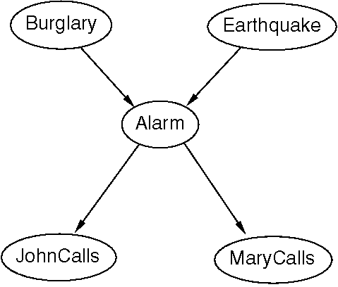
We know that each node stores a probability table as follows:

        NODE                PROBABILITY TABLE
        Burglary            P(B)
        Earthquake          P(E)
        Alarm               P(A|B,E)
        JohnCalls           P(J|A)
        MaryCalls           P(M|A)

We also know that the joint probability distribution over all five variables can be computed as the conformal product of these five probability tables:

        P(B,E,A,J,M) = P(B) * P(E) * P(A|B,E) * P(J|A) * P(M|A)

This joint distribution will contain 32 cells, one for each combination of the five random variables.

Now suppose that we want to compute P(J). We can do this by "marginalizing" the joint distribution. In other words, we sum over all possible values of the other variables:

        P(J) = sum[B,E,A,M] P(B,E,A,J,M)

Remember that in any boldface P formula, we can substitute in any value for the variables that appear in the equation. In this case, we can substitute either J=1 or J=0:

        P(J=0) = sum[B,E,A,M] P(B,E,A,J=0,M)
        P(J=1) = sum[B,E,A,M] P(B,E,A,J=1,M)             (1)

So this shows one way that we could compute P(J). However, it is very expensive, because we must multiply out all of the probability distributions, and this will take time that is exponential in the number of distributions. Is there a cheaper way?

The answer is YES. Consider the following simple example:

        ace + acf + ade + adf + bce + bcf + bde + bdf           (2)

This is a large expression that requires 16 multiplications and 7 additions to evaluation. But we can factor out the common terms a and b and obtain the expression

        a(ce + cf + de + df) + b(ce + cf + de + df)

Notice that the two terms in parentheses are identical, so we can factor them out:

        (a + b)(ce + cf + de + df)

We can do the same thing with the terms involving c and d, and we obtain

        (a + b)(c + d)(e + f)                                   (3)

This requires 2 multiplications and 3 additions, so it is much more efficient. We want to do the same thing with the conformal products.

Now let us return to the problem of computing P(J), which we wrote as equation (1) above. Let us rewrite this in terms of the conformal product of the original probability tables:

        P(J) = sum[B,E,A,M] P(B) * P(E) * P(A|B,E) * P(J|A) * P(M|A)

This has the same structure as our example, equation (2). We are taking a sum of many product terms. But we can "push" the summations inside some of the products and get a formula that looks more like equation (3). For example, consider the term P(M|A). This is the only term that involves M. So we can push the summation over M in to this formula.

        P(J) = sum[B,E,A] P(B) * P(E) * P(A|B,E) * P(J|A) * sum[M] P(M|A)

Let us write

        P[A] = sum[M] P(M|A)

to be the probability table that results from summing over the values of the variable M. We use square brackets to indicate that this probability table is a "potential"; it does not necessarily have an interpretation as a conditional probability distribution. (In fact, in this case, all of its cells will have the value 1.)

The expression we are now trying to evaluate is

        P(J) = sum[B,E,A] P(B) * P(E) * P(A|B,E) * P(J|A) * P[A]

Notice that there are two probability tables involving the random variable E. If we multiplied them together, then we could sum over E. We can write this as

        P(J) = sum[B,A] P(B) * sum[E] [P(E) * P(A|B,E)] * P(J|A) * P[A]

The result of this will be a potential involving only the variables A and B:

        P(J) = sum[B,A] P(B) * P[A,B]  * P(J|A) * P[A]

There are only two probability tables involving the variable B. So we can compute their conformal product and them sum over B to get a table that involves only the variable A:

        P(J) = sum[A] sum[B] [P(B) * P[A,B]]  * P(J|A) * P[A]
        P(J) = sum[A] P[A] * P(J|A) * P[A]

Finally, we must take the conformal product of all three of these probability tables. This will give us a single table P[A,J]:

        P(J) = sum[A] P[A,J]

Now we can sum over A to obtain the answer.

What we have done is to find an efficient factoring of the original expression:

        P(J) = sum[B,E,A,M] P(B) * P(E) * P(A|B,E) * P(J|A) * P(M|A)   
             = sum[A] (sum[B] (P(B) * sum[E] (P(E) * P(A|B,E))) * sum[M] P(M|A))

The largest intermediate probability table that this creates is a table over 3 variables (8 cells). So this is a big savings over creating the full joint distribution. The total number of additions and multiplications will be much less as well.

Turning this into an Algorithm

The SPI algorithm works as follows. We are given a single variable (for example, J) as a query variable, Q, along with a belief network N that involves a set of n variables V = {V1, ..., Vn} and a list of probability tables (ptables) L = (T1 T2 ... Tn):

ASK(N,Q)
  Let M = V \ Q be a list of all variables in N except
  the query variable Q.  These are the variables we will sum
  over. 

  // remove any variables that can be removed by summing over a single
  // table. 
  For each ptable T in L do
     let VT be the variables in T that are also in M.
     let VS be the set of all variables in T that are also in M and do
     not appear in any other ptable in N.  We can sum over these variables:
       T := sum-over(T, VS)
       delete VS from M
  end for

  // main loop
  While L contains more than one ptable do
     let bestPair = NIL
     let bestSize = |M| + 1
     let bestMarginalizers = NIL
     For each pair of ptables (T1, T2) in L do
        compute the list of variables PV that would appear in the
        conformal product of T1 * T2
        determine which of these variables PVS could be summed over
        (because they do not appear in any other ptable in L)
        let Size = |PV| - |PVS| be the number of variables that would
          remain after the summation.
        if Size < bestSize
           bestSize = Size
           bestPair = (T1, T2)
           bestMarginalizers = PVS
     end for
     Let T12 = sum-over(conformal-product(bestPair), bestMarginalizers)
     delete T1 and T2 from L
     insert T12 into L
  end while
     
  print and return the single remaining probability table in L

Handling TELL Operations

To see how to handle TELL operations, let us first consider how we could handle them using the joint distribution. When we are told the value of a random variable, we can take the joint probability distribution and delete all cells in the table that correspond to the other values of the random variable (i.e., the values that were not observed). We then normalize the remaining cells so that the table again sums to 1. Notice that the resulting table no longer mentions the variable that was observed (or equivalently, all of the cells in the table correspond to the same, observed, value of the variable).

We can do something analogous with the belief network representation. When we are told that variable V has value val, we delete all cells involving all other values of of V from all of the ptables in the belief network. These tables now no longer involve the variable V.

However, we do not normalize the ptables (this would be difficult to do). Instead, we normalize the final answer that is printed by the SPI algorithm.

TELL(N,V,val)

  for each ptable T in N do
    if V is one of the variables in T
    T := project(T,V,val)
    if T has no more variables, delete T from N
  end

Change ASK to normalize the final answer before it prints it.