Applications of Heap

The obvious application (and the original motivation) of heap is heapsort:

• heapify: \(O(n)\)
• \(n\) pops: \(O(n \log n)\)

Total time: \(O(n \log n)\). Note that even if you don’t know heapify and replace it with \(n\) pushes, it doesn’t change the overal complexity.

However, heaps can also be used in many other much more interesting scenarios in algorithm design. Here we showcase some classical examples.

\(k\)-way mergesort

We all know mergesort uses binary division. But what if we divide the array \(k\) ways? And then recursively mergesort \(k\) subarrays, and finally combine \(k\) sorted (sub)lists. This is known as \(k\)-way mergesort, a very interesting generalization of the classical mergesort which is a special case with \(k=2\).

• divide: now takes \(O(k)\) time
• conquer: now \(k\) subproblems (\(k\times\))
• combine: how would you combine \(k\) sorted lists?

Again, like classical mergesort, combine is where most of the work lies. Ok, let’s generalize the “two-pointers” idea to “\(k\)-pointers”. But while comparing two numbers is trivial, how do you compare \(k\) numbers and take the smallest one? If you take \(O(k)\) time every step, that would be too slow. Notice that most numbers remain unchanged (only the best number in the previous round is replaced by its successor in that sublist), so you waste much time doing repeated comparisons.

So we use a heap instead!

• First, build an initial heap out of the \(k\) leaders of each sublist (\(O(k)\) time).
• Pop the smallest number from the heap, and replace it with its successor in that sublist (if that list is not empty yet). (\(O(\log k)\) time).
• Repeat until all sublists are empty. (\(n\) iterations, each taking \(O(\log k)\) time because the heap size remains \(k\) with replacements, until at least one sublist is empty and heap size is less than \(k\), but in any case, the heap size is bounded by \(k\)).

So the total time for the combine step is \(O(k + n\log k)=O(n\log k)\) because \(k < n\).

Caveat: Notice that if \(k \geq n\), our \(k\)-way mergesort becomes heapsort! So the two extreme special cases of \(k\)-way mergesort are classical mergesort (\(k=2\)) and heapsort (\(k=n\)).

Now divide+combine (the non-recursive parts, or the work at each level) is \(O(k+n\log k)=O(n\log k)\). Now we get back to the overall time using recurrence:

\[ T(n) = k T(n/k) + O(n\log k)\]

We’ll still use the “recursion tree” method to expand the recursion:

• The first level has work \(O(n\log k)\), with \(k\) branches.
• Each of the \(k\) branches is of size \(n/k\), and each of them in the second level has work \(O(n/k \cdot \log k)\) (still \(k\)-way division, so heap size is still \(O(k)\), only \(n\) becomes \(n/k\)), so the second level has total work \(O(k \cdot n/k \log k) = O(n\log k)\).
• Continue this recursion, you’ll see that each level has work \(O(n\log k)\).
• How many levels? Because each node has \(k\) branches, so the height is \(h=\log_k n\).
• Total work: \(O(n\log k \cdot \log_k n) = O(n\log k \cdot \frac{\log n}{\log k}) = O(n\log n)\).

This is a remarkable result that the runtime of \(k\)-mergesort does not depend on \(k\)!

Alternative method: Using the Master Method, we can see that the above recurrence falls into case 2, so \(T(n)=O(n\log n)\).

Team selection problem

Another problem similar to \(k\)-way mergesort is the team selection problem: the United States have \(n=50\) states, and each state has selected its (sorted) top \(k\) tennis players. Now we need to select the top \(k\) players to form team USA (for Olympics). How would you do that as fast as possible?

Same as \(k\)-way mergesort, you build an initial heap of size \(n\) from the best players of each state. Then you pop/push (or heapreplace), until you have popped \(k\) players.

Time: \(O(n + k\log n)\), because the heap size is bounded by \(n\).

Can you make it even faster? Well, if \(k \ll n\), a key observation is that the vast majority of states will have no representatives on team USA. If a state’s best player can’t make the top \(k\) in the initial heap of size \(n\), then every player from that state doesn’t have a chance in team USA. For example, if \(k=5\), team USA will likely have (even multiple) players from big states like California and New York, and nobody from most other states. This observation suggests we should narrow down our initial heap to just the top \(k\) (best among the best) players (or states) from the \(n\) top players from each state. So we use quickselect to select the \(k\)th best player among those \(n\) leaders and scan all those \(n\) leaders again to select the top \(k\) leaders. Now you build an initial heap of just \(k\) players, and because the heap size is bounded by \(k\), you improve the total time to:

\[ O(n + k + k\log k)=O(n+k\log k)\]

which is slightly faster than \(O(n+k\log n)\).

\(n\)-best pairs problem

A slightly more involved problem is \(n\)-best pairs problem. Given two unsorted lists \(A\) and \(B\), each with \(n\) integers, their cross-product (or Cartesian product) is \(n^2\) pairs:

\[ A\times B = \{ (x, y) \mid x \in A, y \in B \} \]

How to select the \(n\) smallest pairs from \(A\times B\)? Let’s say we compare pairs by their sums:

\[ (x,y) < (x',y') \text{ iff. } x+y < x'+y' \text{ or } x+y==x'+y' \text{ and } y<y' \]

i.e., between two pairs, the one with the smaller sum is considered smaller, or in the case of a tie, the pair with smaller second dimension wins (actually you can define this relation arbitrarily, as long as it’s monotonic). For example:

>>> a, b = [4, 1, 5, 3], [2, 6, 3, 4]
>>> nbest(a, b) 
[(1, 2), (1, 3), (3, 2), (1, 4)]

Let’s start with the most obvious idea, and gradually improve it.

• Method 1: Naiveily, you would enumerate all \(n^2\) pairs, sort them (\(O(n^2 \log n^2)=O(n^2\log n)\)), and return the first \(n\) in the sorted array; total time: \(O(n^2 + n^2\log n + n) = O(n^2 \log n)\).
• Method 2: Can we make it a bit faster? Well, we don’t need the total ordering of these \(n^2\) pairs, so we can use quickselect instead. But some students would call quickselect \(n\) times (let’s say AB is the array of \(n^2\) pairs): first qselect(AB, 1) for the smallest pair, then qselect(AB, 2) for the 2nd smallest pair, all the way to qselect(AB, n) for the \(n\)th smallest pair. That would be too slow (in fact, even worse than naive: \(O(n^2 + n \cdot n^2)=O(n^3)\)). Actually, you only need to call quickselect once – just use qselect(AB, n) to establish the threshold, and then scan the whole array again to output every pair that is smaller than the threshold. Total time: \(O(n^2 + n^2 + n^2)=O(n^2)\) which is slightly better than naive.
• Method 3: Now let’s really make it a LOT faster. Following \(k\)-way mergesort and team selection, we know that it is better to have the sublists sorted so that we can use heap. Therefore, let’s sort a and b first. Once they’re sorted, obviously \((a_0, b_0)\) is the smallest pair. But who’s the second best? Well, it must be either \((a_0, b_1)\) or \((a_1, b_0)\). Let’s say that \((a_0, b_1)\) is the second best, which gets popped. Then we would push its own successors, \((a_0, b_2)\) and \((a_1, b_1)\). So in general, once we pop \((a_i, b_j)\), we need to push two successors, \((a_i, b_{j+1})\) (if \(j+1<n\)) and \((a_{i+1}, b_j)\) (if \(a+1<n\)). We use a heap to store the candidates for the next best (the frontier of expansion), which starts with only one pair. The size of the heap is bounded by \(n\) because each time you pop one and push at most two, so the size increase by (at most) 1 per step. Therefore, total time is \(O(n\log n + n\log n + n\log n)\) where the first two terms are sorting and the last one is \(n\) heappops/heappushes.

Caveat: if a successor is already in the heap, don’t push it twice. This means you need some hash-based datastructures such as Python set to check whether some pair is already pushed, in \(O(1)\) time.

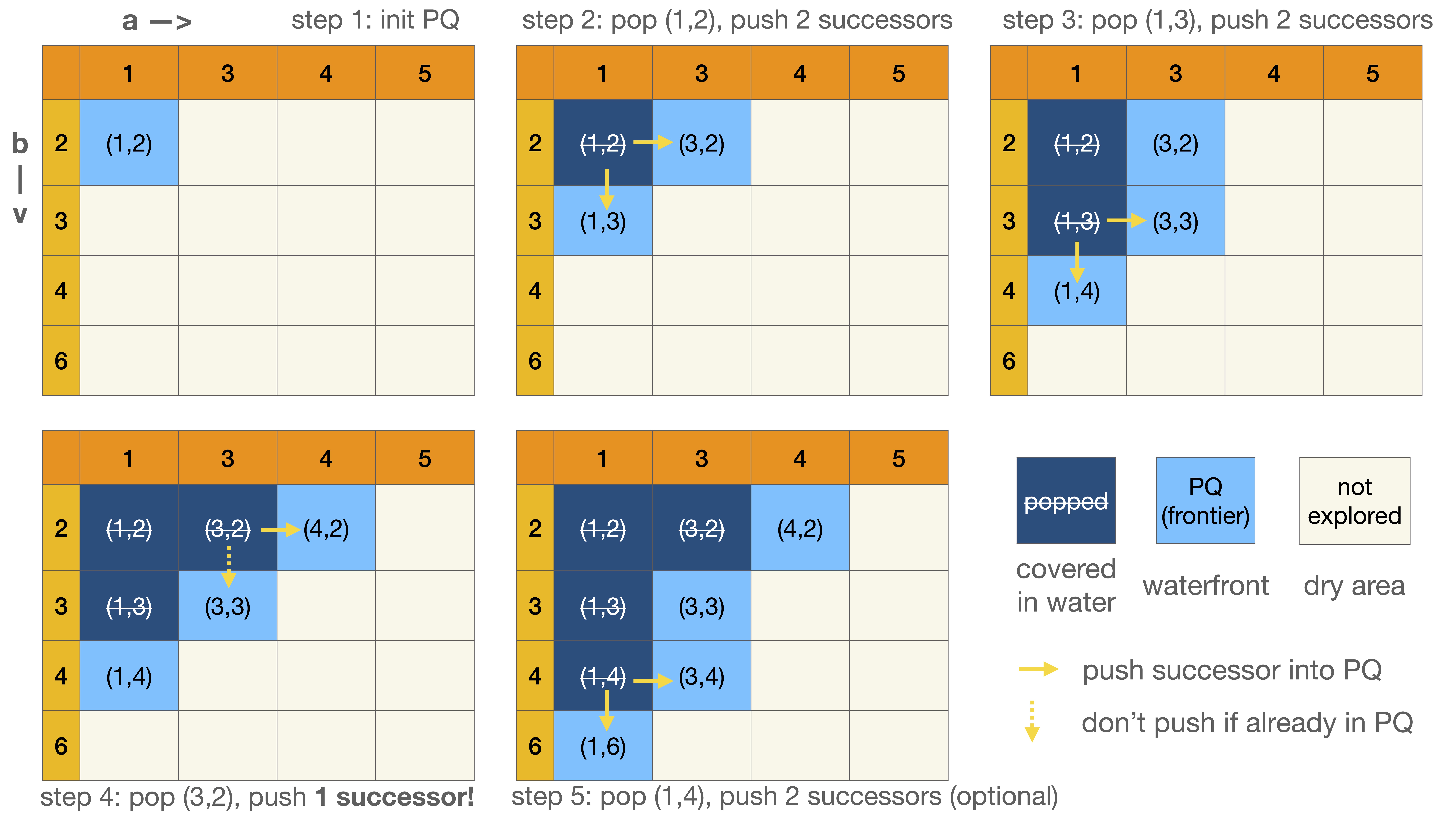
Here is a picture:

You can imagine in a flooding zone, water level keeps rising. Initially, water will only cover the top-left corner (lowest area) and gradually cover more and more cells. Those covered in water are already popped from the heap, and the “waterfront”, i.e., the frontier of expansion, is the current heap, which marks the boundary between those already popped and those never pushed (dry area). In the end, you can see that among \(n^2\) cells, most are never explored (not even computed), i.e., in the dry area, and only \(n\) are popped, i.e., submerged in water, and \(n\) are in the frontier. That’s why this algorithm is so efficient.

Alternative method: Instead of starting with just the top-left corner (\((a_0, b_0)\)), you can also start with all the first column \(\{(a_0, b_0), (a_1, b_0), \ldots, (a_{n-1}, b_0)\}\), and then you just need to pop/push (or heapreplace) instead of pop one and push two. Note that this method is much more similar to team selection (each \(a_i\) is a “state”, with its sorted best players being \((a_i, b_0), (a_i, b_1), \ldots\)). In this case, a does not need to be sorted (but b must be sorted; or vice versa if you start with the first row). The other small advantage is that you don’t need to maintain a set to check if some pair is already pushed. Total time: \(O(n\log n + n + n\log n) = O(n\log n)\); the first term is sort b, the second is heapify, and the third is \(n\) heappops. Same runtime, just not as pretty (or symmetric) as the above method, but may be a bit easier to implement.

\(k\)-smallest numbers in a datastream

Historical Notes

The \(n\)-best problem is taken from my \(k\)-best parsing paper (Huang and Chiang, 2005).