So far we have been using the recursion tree method to analyze the complexities of divide-n-conquer algorithms. But you likely have heard of the other widely used method, the Master Theorem, which was popularized (as the “Master method”) by the CLRS textbook. With this method, you don’t need to draw the recursion trees; instead you only need to decide which of the three cases this recursion falls into, and look up the answer. Therefore you can think of it as a mnenomic or “cookbook” method.

Our objective in this section is to give you a quick and gentle introduction to this powerful method by deriving it from the recursion tree method, so that you can understand the geometric intuition behind this theorem rather than memorize the details. Therefore the treatment of math here is rather informal (missing a lot of details). For a much more rigorous treatment, please refer to CLRS or Wikipedia.

General Form of Recurrence

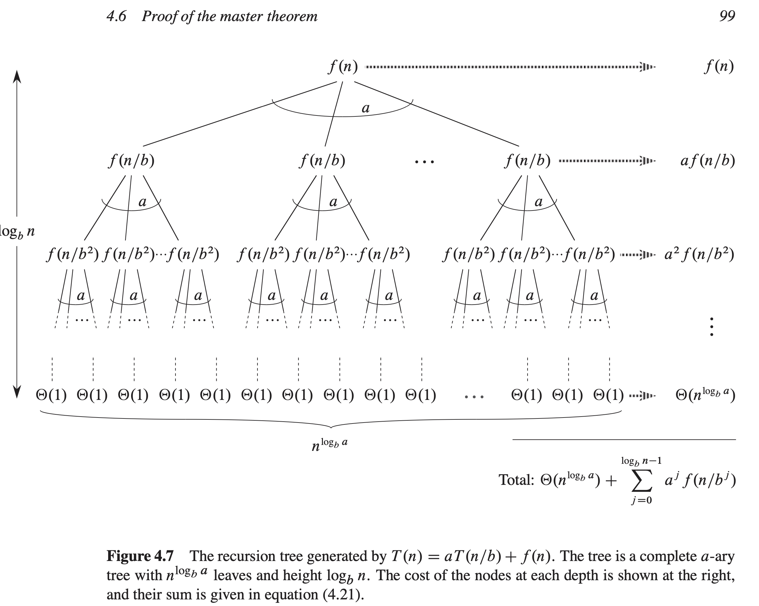
For a general divide-n-conquer algorithm, we divide a problem of size \(n\) evenly into \(b\) non-overlapping subproblems (each with size \(n/b\)), and conquer \(a\) of them. Together with the non-recursive work (i.e., divide + combine) of \(f(n)\), we can write the recurrence as

\[T(n) = aT(n/b) + f(n)\]

For example, in mergesort, \(a=b=2\) (conquer both children) and \(f(n)=n\), while in binary search, \(a=1\), \(b=2\) (conquer one of the two children), and \(f(n)=1\). Note that:

• \(a\) is the branching factor of the recursion tree, so \(a\geq 1\);
• \(b\) is the problem division factor, so \(b>1\) (the problem size must shrink otherwise it’ll be an infinite recursion);
• For the scope of this book, we assume \(a\leq b\) (conquer a subset of subproblems), but the Master Theorem works for \(a>b\) as well.
• \(a\) and \(b\) are constants; so technically speaking, we can’t apply Master Theorem for \(k\)-way mergesort (\(T(n)=kT(n/k) + n\log k = \Theta(n\log n)\)) where \(k\) is a variable (although it would be a perfect fit for case 2 below).

Amount of Work Per Level and the Three Cases

Recall that the key to the recursion tree analysis is the amount of work per level (see below a recursion tree from CLRS, Fig. 4.7):

• The first level has \(f(n)\) work;
• The second level has \(a\) nodes, each with \(f(n/b)\) work, so total \(a\times f(n/b)\) work;
• At level \(h\) (\(h=0\ldots \log_b n\)), we have \(a^h\) nodes, with each node (being size \(n/b^h\)) having \(f({n}/{b^h})\) work, so total \(a^h \times f({n}/{b^h})\) work;
• Finally, the tree has height \(\log_b n\), and at the last level, we have \(a^h = a^{\log_b n} = a^{\frac{\log_a n}{\log_a b}} = n^{1/\log_a b} = n^{\log_b a}\) leaf nodes, each with work \(f(1)=O(1)\). So total \(n^{\log_b a}\) work.

Now we can ask the key question that divides the analysis into three cases: does the amount of work per level grows or shrinks as you get deeper? Or (more or less) equivalently, which one dominates the other, the root work \(f(n)\) or the leaves work \(n^{\log_b a}\)?

• Will each level of the recursion tree have more work than the previous level? If so, the tree will have exponentially more work as it gets deeper (“exponential explosion”), and the final level, which are made of all leaf nodes, will dominate the computation. The sum of work is a growing geometric series (from root to leaves), but the inverse series (from leaves to root) is a converging geometric series. Therefore \(T(n)=\Theta(a^h f(1))=\Theta(n^{\log_b a})\). We call this case “leaf-heavy”.
• Will each level of the recursion tree have the same amount of work? If so, each level will have the same \(f(n)\) work, and the total amount of work will be simply \(f(n)\) times the height of the tree (which is \(\log_b n\)). Therefore \(T(n)=\Theta(f(n) \log_b n)\). This height is the source of all \(\log n\) factors in the complexities you’ve seen so far.
• Will each level of the recursion tree have less work than the previous level? If so, the tree will exponentially less work as it gets deeper (“exponential decay”), and this geometric series will converge to the same complexity as the work in the root node (which is \(f(n)\)). Therefore \(T(n)=\Theta(f(n))\). We call this case “root-heavy”.

Here are the pictures (all you need to remember are these geometric intuitions!):

• leaf-heavy (triangle): growing geometric series, converging to leaves (\(a^h = n^{\log_b a}\)); think balanced binary tree traversal:

            *                    f(n)
        *       *             a f(n/b) > f(n)
      *  *    *   *         a^2 f(n/b^2) >> f(n)
           ...                 ...
**************************  a^h f(1) >>>>>> f(n)

• equal (rectangle): area is \(f(n) \times h= f(n)\log_b n\); think mergesort:

    *******************          f(n)
    ********* *********        a f(n/b) = f(n)
    **** **** **** ****      a^2 f(n/b^2) = f(n)
            ...                 ...
    *******************      a^h f(1) = f(n)

Another typical example: binary search (\(a=1, b=2, f(n)=1\)):

  *        f(n)   = 1
  *      a f(n/b) = 1
 ...      ...
  *      a^h f(1) = 1

• root-heavy (upside-down triangle): shrinking geometric series, converging to the root $f(n); think quickselect best case:

**************************       f(n)
      *************            a fn/b) < f(n)
         *******             a^2 f(n/b^2) << f(n)
           ...                  ...
            *                a^h f(1) <<<<<< f(n)

More formally, where do we draw the boundary? Well, we either compare the root \(f(n)\) with the leaves \(n^{\log_b a}\) to see which one is smaller, or compare the first two levels \(f(n)\) and \(af(n/b)\) to see which one grows faster. Either way, you can get the same threshold \(n^{\log_b a}\) as the critical polynomial that demarcates the boundaries of the three cases. A technical detail is that you need to leave a small polynomial margin of \(n^\epsilon\) between the three cases (so that the boundaries are more widely marked):

• leaf-heavy: if \(f(n)=O(n^{\log_b a - \epsilon})\) for some constant \(\epsilon > 0\), then \(T(n)= \Theta(n^{\log_b a})\);
• equal: if \(f(n)=\Theta(n^{\log_b a})\), then \(T(n)=\Theta(f(n) \log_b n)\);
• root-heavy: if \(f(n)=\Omega(n^{\log_b a + \epsilon})\) for some constant \(\epsilon > 0\) and if \(f(n)\) satisfies some “regularity condition” which holds for most functions we encounter, then \(T(n)=\Theta(f(n))\).

Case 1: leaf-heavy

Examples:

Note: for heapify, \(f(n)=\log n\) grows slower than any polynomial \(n^c\) with \(c>0\), so it definitely is dominated by \(n^{\log_b a} = n\).

Case 2: equilibirium

Examples:

Note: \(k\)-way mergesort should belong to this case although \(k\) is a variable here. We need to (slightly) genearalize the scope of this theorem by allowing \(a\) and \(b\) to be variables that do not change with height, and we need to use my form of \(T(n)=\Theta(f(n)\log_b n)\) rather than the textbook result of \(T(n)=\Theta(f(n)\log n)\) because the former works even when \(b\) is a variable that doesn’t change with height. But this is a rather minor point.

Case 3: root-heavy

Examples:

Note: in most divide-n-conquer instances, \(b=2\) and \(a\in{1,2}\), so the critical threshold is \(n^0=1\) or \(n^1\). Any \(f(n)\) that grows faster than \(n\) falls into this root-heavy case, i.e., \(T(n)=2T(n/2) + n^2\log n = \Theta(n^2\log n)\).

Caveats

1. Note that there are “gaps” between the three cases. In case 1, \(f(n)\) not only needs to be smaller than \(n^{\log_b a}\), it needs to be polynomially faster, i.e., by a small factor of \(n^\epsilon\). Similarly, in case 3, \(f(n)\) not only needs to be bigger than \(n^{\log_b a}\), it needs to be polynomially bigger, i.e., by a small factor of \(n^\epsilon\). So there are gaps between case 1 and case 2, and between case 2 and case 3 (\(f(n)\) is bigger than \(n^{\log_b a}\) but not polynomially bigger).
2. In the gap between case 2 and case 3, a very common case is \(f(n)=\Theta(n ^{\log_b a} \log^k n)\) for some constant \(k>1\), e.g., \(T(n)=2T(n/2) + n\log n\). A more generalized version of case 2 can include these cases, under the same “rectangle picture” even though technically speaking each level has slightly more work than the previous level, but \(\log^k n\) grows extremely slowly. This would still solve to \(T(n) = \Theta(f(n) \log_b n)\). So \(T(n)=2T(n/2) + n\log n = \Theta(n \log^2 n)\). Another example: \(T(n)=T(n/2)+\log n = \Theta(\log^2 n)\) (the only NOT COVERED case in the big table below). See Wikipedia for more details (this part is not covered in CLRS).

Table of Common Recurrences and Examples

The biggest drawback of Master Theorem is that it can not handle non-even (esp. worst-case) divisions such as \(T(n)=T(n-1) + f(n)\) which are very common in datastructures (e.g., quicksort/quickselect worst-case). Those cases can still be solved by the recursion tree method, which is more flexible (and thus the default method). Here I summarize the 3x3 combinations of

• the three most common divisions:

  • \(T(n) = T(n/2) + ...\)
  • \(T(n) = 2T(n/2) + ...\)
  • \(T(n) = T(n\!-\!1) + ...\)

• and the three most common \(f(n)\)’s:

  • \(f(n) = 1\)
  • \(f(n) = \log n\)
  • \(f(n) = n\)

These combinations cover the vast majority of the most commonly used divide-n-conquer instances in algorithms and datastructures, so it’s worthwhile to list all of them:

Historical Notes

The Master Theorem was published by Bentley, Haken, and Saxe in 1980.