Backtracing for the Best Solution

In the above section we showed how to compute the best value of the MIS problem:

\[f[i] = \max\{f[i-1],\quad f[i-2] + a_i\}\]

with

\[ f[-1] = f[-2] = 0\]

E.g., for the example problem

9---10---8---5---2---4

We can figure out the best value of \(21\). But how to find the optimal subset that adds up to \(21\) (which in our case is \([9, 8, 4]\))?

For all optimization problems, you often need to find the optimal solution, not just the optimal value. Knowing the former implies the latter but not the other way around. For example, in shortest-path problems, it’s not enough to know “the best route from city A to city B take 1.5 hours”; instead, you need the best route itself, like “city A -> city C -> city D -> city B”.

Method 0 (non-DP): Recursion with Byproduct

Before discussing how to do it in DP, let’s first try to do it in exhaustive search, which prepares us for the DP version. Recall our recursive function:

def mis2(a):
    def _mis(i):
        if i < 0: return 0 # empty
        return max(_mis(i-2) + a[i], 
                   _mis(i-1))
    return _mis(len(a)-1)

To return the optimal subset, we “tag it along” the above recursion, using the “recursion with byproduct” idea from Sec 1.5:

class mypair(tuple):
    __add__ = lambda a,b: (a[0]+b[0], a[1]+b[1])

def mis6(a):
    def _mis(i):
        if i < 0: return mypair(0, [])
        return max(_mis(i-2) + (a[i], [a[i]]),
                   _mis(i-1))
    return _mis(len(a)-1)

The helper function _mis() now returns a pair (mypair), the best value and the best subset, and the new summary operator \(\oplus\) takes the max of two pairs (compared using their values) instead of two numbers. Note that the combine operator \(\otimes\) (+ on line 7, which calls the __add__ function on line 2) has been overloaded in the mypair class to serve our purpose (I could’ve used * instead of + to be more semiring-like). This gives rise to the first and very bad method of returning the best solution in DP.

Python Caveat: it’s impossible to change a builtin function such as tuple.__add__, so we have to wrap around tuple by a user-defined (sub)class.

Method 1 (very bad): Storing the best subsolutions

Like the above solution, the naive method to retrieve the best solution in DP is just to store the best subsolution for every subproblem, and therefore the subsolution for the global subproblem is indeed the global solution:

\[f[i] = \oplus \{f[i-1], \quad f[i-2] \otimes (a_i, [a_i])\}\]

with

\[ f[-1] = f[-2] = (0, []) \]

Note the summary \(\oplus\) is max in Python, and the combine operator \otimes is the __add__ (operator overloading) defined above.

This sounds trivial (and can be done beautifully with operator overloading like we did above), but is actually a very bad method that you should NEVER use. Unfortunately, in my teaching career, every year, many students still use this naive method without realizing how much overhead it causes. So let’s take a moment to analyze.

Space complexity: Previously, you only need to store the best value for each subproblem, so \(O(n)\). Now you need to store the best subsolution for each subproblem as well, which costs \(O(n^2)\) since each subsolution is a list of at most \(\lceil n/2 \rceil\).

Time complexity: Previously, the time compplexity is \(O(n)\) because each subproblem involves a max over two values. Now, you need to create (and save) the best subsolution, which costs \(O(n)\) for subproblem, so total \(O(n^2)\). Important: note that we need to create new lists like the __add__ above rather than appending to the existing list, otherwise later subproblems will destroy the subsolutions stored for earlier subproblems.

So both time and space become much worse with this method, and this is true for all DP instances. So you should never use this method even though it’s conceptually simple, easy to program, and easy to debug. Instead, you should by default use the following method of backpointers.

Method 2 (default): Backpointers and backtracing

Think again about divide-n-conquer. You now know the best value of the global problem (\(a_1, \ldots, a_n\)), so you should also backtrace from the global problem. But unlike divide-n-conquer, now we need each subproblem (including the global one) to tell us how to best divide that subproblem, because there are multiple ways of division (in our case, either dividing into \(f[i-2]\) and \(a_i\) or dividing into \(f[i-1]\)). This is the crucial difference between DP and divide-n-conquer:

DP is divide-n-conquer with multiple ways of division.

To remember the best division for each subproblem, we need another table \(b[i]\), to store the backpointers, which record for each \(i\), where or how the best value of \(f[i]\) is obtained. In our case, \(f[i]\) involves a choice between two cases, so \(b[i]\) only needs to be a boolean like this:

\[ b[i] = (f[i] \neq f[i-1])\]

Therefore, \(b[i]=T\) means the best solution of \(f[i]\) is to take \(a_i\), i.e., \(f[i]=f[i-2]+a_i\), and \(b[i]=F\) means the best solution of \(f[i]\) is not to take \(a_i\), i.e., \(f[i]=f[i-1]\). With this backpointers table, we can backtrack from the global problem \(f[n]\) backwards to base cases. This process is just like doing top-down recursion again, but this time each subproblem has a deterministic divide, just like normal divide-n-conquer:

• start with \(i=n\) (global)
• if \(b[i]=T\), it means \(f[i]=f[i-2]+a_i\), so take \(a_i\), and backtrack to \(i-2\).
• if \(b[i]=F\), it means \(f[i]=f[i-1]\), so don’t take \(a_i\), and backtrack to \(i-1\).
• until reaching a base case (\(i<1\)).

Here is the complete table for the running example. Note that \(f[i]\) and \(b[i]\) is computed left-to-right (forward pass) while the last row is computed right-to-left (backward pass).

It is crucial that you understand the following points:

• \(b[i]=T\) does not mean \(a_i\) is included in the global best solution; it only means \(a_i\) is included in the local best solution (for subproblem \(f[i]\)). For example, \(b[1]=T\) but \(a_1=10\) is not included in the global solution because it’s bypassed in the backtracking.
• \(b[i]=F\) means \(a_i\) is not included in the local best solution, but it is also guaranteed that \(a_i\) is not included in the global best solution, because even if the global best solution happens to visit \(f[i]\), we still won’t take \(a_i\) (see \(a_3=5\) in this example).
• whether \(a_i\) is included in the global best solution can not be decided in the forward pass, and can only be decided in the backward phase.

Complexities: both space and time complexities remain \(O(n)\), so the overhead is only a constant factor.

Method 3 (advanced): On-the-fly recomputing

(advanced topic, to be completed)

Graph Interpretations of MIS, Fibonacci, and bitstrings

All DP algorithms have graph interpretations, which most textbooks ignore, but I found them quite helpful in student learning. In fact, many students told me (at the end of my course) that in retrospect, I should have taught graph algorithms first, and then DP wuold have been much easier with graphs in mind.

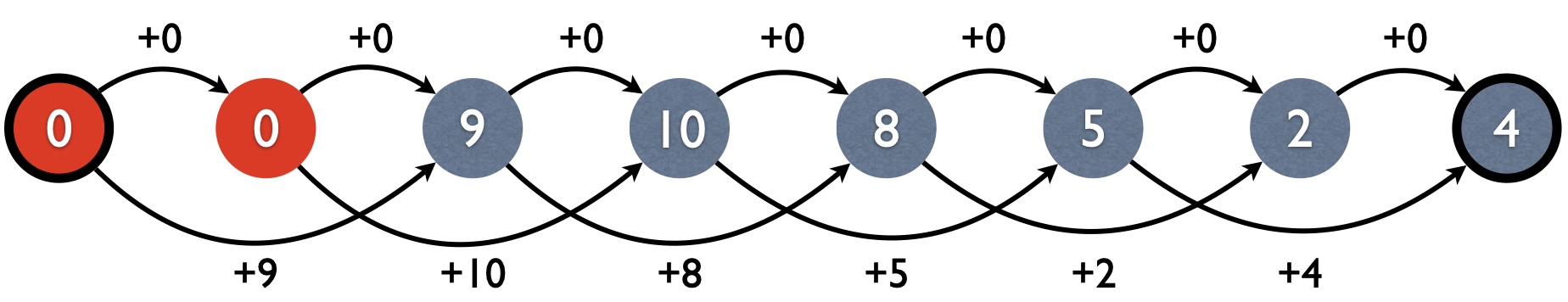
The graph interpretation of MIS is simply to find the longest path in this induced graph below:

Note that the induced graph (also known as the “DP graph”) is often quite different from the input graph (if the input is a graph). In our case, the input graph is a linear-chain undirected graph, but the induced graph is a directed (acyclic) graph. The induced graph closely resembles the DP recurrence. Here each node has two incoming edges, one with +0 from the previous node i-1 (not taking a[i]), and the other with +a[i] from node i-2 (taking a[i]). More importantly, there is a “summary” operator associated with each node; in our case, it’s max (but you will see below that it will be + for the other two problems).

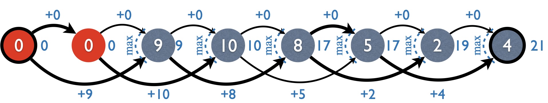
The backpointers can be interpreted as a marker for the best incoming edge for each node, which we mark as bold in the above graph. Then backtracing is simply following these bold edges backwards from the end.

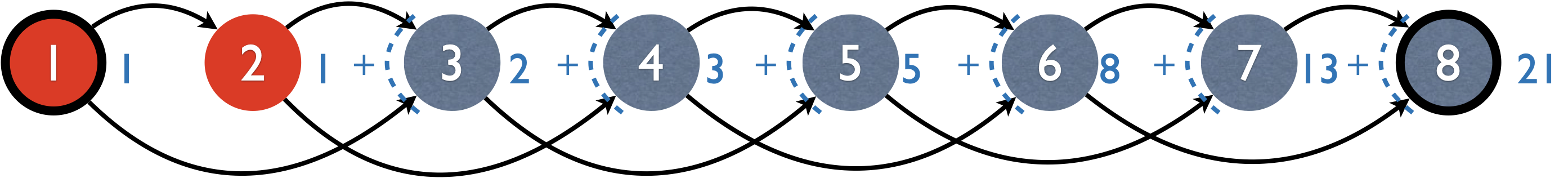
Now what about the graph interpretation for Fibonacci and bitstrings? Instead of longest path, here we count the number of paths. Therefore, the induced graph is unweighted (i.e., no cost on edge as we care about the number of paths rather than the cost of a path), and the “summary” operator is +.

You can also see that MIS is an optimization problem (with the summary operator being a comparison, min or max) whereas Fibonacci and bitstrings are non-optimization problems (counting) with the summary operator being + (and no backpointers are needed). Yes, DP can solve both types of problems.