
Recall that the secret of DP is:
divide-n-conquer = single divide into non-overlapping subproblems
DP = divide-n-conquer with multiple divides
In the last section, our examples are all about unary (incremental) divides, but the more exciting divides are binary ones such as mergesort or quicksort best-case. In this section, we will explore the DP instances of such binary-divide recursions.
The simpliest example in this category is the number of \(n\)-node BSTs. For example,
n=0: 1 (empty tree)
n=1: 1 (singleton)
n=2: 2 (1->2 or 1<-2)
n=3: 5 (1->2->3, 1->(2<-3), 1<-2->3, 1<-2<-3, (1->2)<-3)

        1        1             2           3          3
         \          \        /   \       /         /
           2           3    1     3     2       1
             \       /                /           \
              3     2                1             2
How to count these numbers \(B(n)\) for an arbitrary \(n\)?
Hint: in the quicksort section, we discussed its connection to BSTs: the recursion tree of quicksort is a BST, with the pivot as the root. Does this give you any idea?
Yes, the difference is that in this problem, the pivot is non-deterministic: it can be anywhere from 1 to \(n\), exactly like our analysis of average-case quicksort. You just need to try all possible partitions. Indeed, that analysis uses DP ideas, although we didn’t elaborate on this connection back then.
For any pivot \(i=1\ldots n\) as the root of BST, we divide this \(n\)-node problem into two subproblems:
Combining them, a pivot of \(i\) would result in \(B(i-1) \otimes B(n-i)\) BSTs. Here the combination operator \(\otimes\) is \(\times\) because any BST on the left can be combined with any BST on the right.
That’s the case of one divide. What about the different divides? Yes, summarize them with the new summary operator \(\oplus\)! In our case, \(\oplus\) is clearly \(+\). So:
\[ B(n) = \oplus_{i=1\ldots n} [B(i-1)\otimes B(n-i)]\]
Base case? Only \(B(0)=1\) is needed; everything else including \(B(1)\) can be derived from it using the recurrence.
Time complexity? Obviously \(O(n^2)\).
Note that this problem is not only our first binary-branching DP example, but also the first DP that has multiple (more than two) divides per (sub)problem (\(\oplus_{i=1\ldots n}\)). The three examples in the previous section are all unary branching with two divides per (sub)problem. So this problem greatly expands our view on DP, and is by far a better representative of DP.
This \(B(n)\) series is actually a famous concept in mathematics: the Catalan numbers. There are numerous interpretations of Catalan numbers (besides our number of BSTs), all related to beautiful recursions. Here are just a few of them:
See more on Wikipedia.
Here we want to discuss one interpretation: the number of (balanced) bracketings with \(n\) pairs of parentheses. For example:
n = 0: 1 bracketing
n = 1: 1 bracketing:  ()
n = 2: 2 bracketings: (()) or ()()
n = 3: 5 bracketings: ((())) or (()()) or ()()() or (())() or ()(())
Or equivalently, in terms of mountain plots where / is
( or push stack and \ is ) or pop
stack:
n = 1: /\

n = 2:
       /\
      /  \  /\/\

n = 3:
       /\
      /  \    /\/\            /\        /\
     /    \  /    \  /\/\/\  /  \/\  /\/  \
Although the 1-1-2-5 sequence matches number of BSTs perfectly, it’s not very obvious to see the connection between the two problems.
Here is a first attempt to solve this problem recursively (and by DP):
Let \(P(n)\) be the number of
bracketings with \(n\) pairs of
parentheses. We divide this problem into the following two cases
depending on whether the leftmost ( and the rightmost
) form a matching pair:
(****) where the outermost ( and
) match and now the problem is reduced to a smaller
subproblem \(P(n-1)\), e.g., to compute
P(3), you first compute (P(2));( and rightmost ) do not
match; so we split these \(n\) pairs
into the left \(i\) balanced pairs
(\(0<i<n\)) and right \(n-i\) balanced pairs. this means we split
into subproblems \(P(i) \times
P(n-i)\), e.g., to compute P(3), you decompose into:
++---- where the ++ is P(1)
and the ---- is P(2)----++ where the ---- is P(2)
and the ++ is P(1)However, you quickly realize this scheme overcounts:
\[P(3) = P(2) + [P(1)P(2) + P(2)P(1)] = 2 + [1\cdot 2 + 2\cdot 1] = 6\]
Why? Because the second case (split) overcounts the
()()() case, which is covered by both ++----
and ----++:
()()()
++----
----++
That’s a big problem! How to fix that?
Well, we need a completely new (and slightly less intuitive)
recursion. Instead of asking whether the outermost parentheses match, we
now ask the rightmost ): which ( do you want
to match? Or equivalently, how many pairs of parentheses are there
between the matching ( and the rightmost ),
including themselves? If the answer is \(n\), then the outermost parentheses match.
If the answer is 1, then the rightmost () match. In any
case, if there are \(i\) \((1\leq i \leq n)\) pairs of parentheses
between the rightmost ) and its matching (,
then we can divide into two subproblems:
( of the rightmost ): \(P(i-1)\);( and rightmost ): \(P(n-i)\).Here is a picture of this new decomposition:
*****(^^^^^)
 i-1   n-i
Now we arrive at the exact same equation as the number of BSTs:
\[P(n) = \sum_{1\leq i \leq n} P(i-1) \times P(n-i)\]
Note: This contrast between our first, overcounting, attempt and the the correct solution is very important. In fact, it will show up again in our discussion of RNA folding, a more advanced DP problem, where the first attempt is known as “CKY” and the second one as “Nussinov”.
Question: now can you align the five BSTs for \(n=3\) with the five bracketings?
A recursion like this can be easily extended to solve many similar problems, such as
Caveat: the average height of BST (also discussed in Sec.
1.2), however, requires a much more complex recursion, because you need
the max operator to determine the height based on subtree
heights, but those heights are themselves random variables. Only knowing
their mean values is not enough to calculate the max
between them accurately. You would end up undercounting the height.
We said each DP algorithm has a graph interpretation. But actually, for binary-branching DP, we need to extend the concept of graph to a slightly more general concept called hypergraphs. In a graph, each edge connects one node to another node. This would be enough for unary branching DP, because each node is a subproblem, and one subproblem reduces (in one divide) to a smaller subproblem. However, in binary branching DP, a problem is divided into two or more subproblems (in each divide). Therefore, we need a hyperedge to connect several nodes (subproblems) into one node.
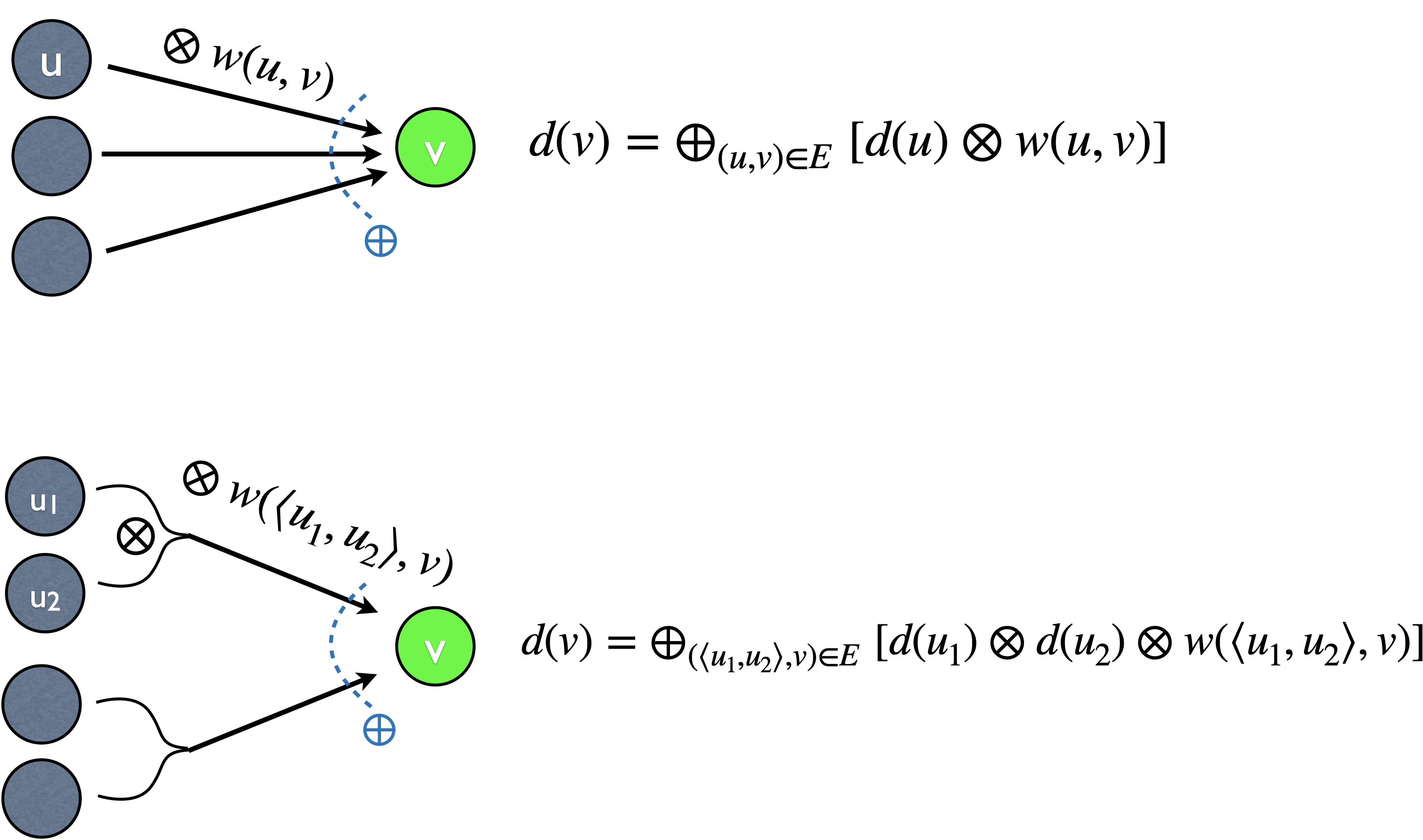
In our BST example, each node \(B(n)\) has \(n\) incoming hyperedges, and each such hyperedge is binary, combining \(B(i-1)\) and \(B(n-i)\) into \(B(n)\). Now you can see that the combination operator \(\otimes\) is naturally associated with each hyperedge, and the summary operator \(\oplus\) is associated with each node. This framework is also equivalent to an AND-OR graph, where each hyperedge is an AND-node and each node is an OR-node.
Also note in the above figure, for completeness, I added edge weigths \(w(u,v)\) and hypereedge weights \(w(\langle u_1, u_2\rangle, v)\). For example, in MIS, the edge weights are \(w(i-2, i)=a[i]\) and \(w(i-1, i)=0\). In the BST example here, the hyperedge weight is 1 (\(\times 1\)).
Most textbooks do not teach the concept of hypergraphs. Instead, they call this type of branching instances “DP over intervals” (such as RNA folding). That interpretation, however, is far too narrow and does not show the real picture. For example, the BST problem here can’t be interpreted as “intervals” because there is no interval here (our \(B(\cdot)\) is a unary function).
In later sections we will see more instances of DP over hypergraphs, which do use intervals \([i,j]\) to define subproblems:
You will see that these seemingly unrelated problems are all equivalent in the hypergraph framework.
I hope my point is clear so far: we should view DP from an abstract point of view, which unifies many different problems in the same framework. The two advanced concepts introduced so far, semiring (with two operators \(\otimes\) and \(\oplus\)) and hypergraph, are the most powerful tools to understand DP in a deep and unifying way.
The hypergraph view of DP is a classical idea discussed by many authors. See also my tutorial on DP under semiring and hypergraph frameworks.