Let’s face it: DP is just hard, much harder than data structures or divide-n-conquer. But on the other hand, it’s also one of the most important, most useful, and cleverest inventions in the history of humanity. If you need to show off human civilization to an alien, then DP is definitely on your list, along with the theory of relativity, formal language theory, Bach and Mozart’s music, etc. Without DP, the human civilization wouldn’t have existed the way it is today, simply because everything you do on your phone uses some DP algorithm behind the scene (such as Viterbi or FFT).

While most textbooks start the DP chapter by classical examples such as LIS/LCS and scheduling, I still found them a bit too complex for beginners. Instead, I use a much simpler example to introduce DP to first-time learners, and hopefully you’ll find this introduction gentler and friendlier.

Example 1: Fibonacci

Naive Fibonacci is Exponential Time

The simplest example I can find for DP is the Fibonacci series:

\[ f(n) = f(n-1) + f(n-2)\]

Wait, why is that relevant to DP? Well, because if you implement it as is (i.e., recursively):

def fib(n):
    return 1 if n <= 2 else fib(n-1) + fib(n-2)

It will be much too slow for even very small numbers like n=50 (which takes >1h on my Mac). In fact, you can see that the time to compute fib(n) grows so fast that it looks like exponential growth:

>>> for i in range(10,41,5):
       t = time.time()
       print(i, fib(i), "%.4f" % (time.time() - t))

10 55 0.0000
15 610 0.0001
20 6765 0.0011
25 75025 0.0129
30 832040 0.1414
35 9227465 1.4998
40 102334155 16.7113

You can see that the runtime increases by \(\times10\) or more while \(n\) increases by +5. This is definitely (at least) exponential, i.e., \(O(a^n)\) for some constant \(a\), instead of polynomial \(O(n^a)\). The difference between polynomial and exponential is indeed the most important division in complexity classes, and is at the very heart of the central problem in computer science: P vs. NP.

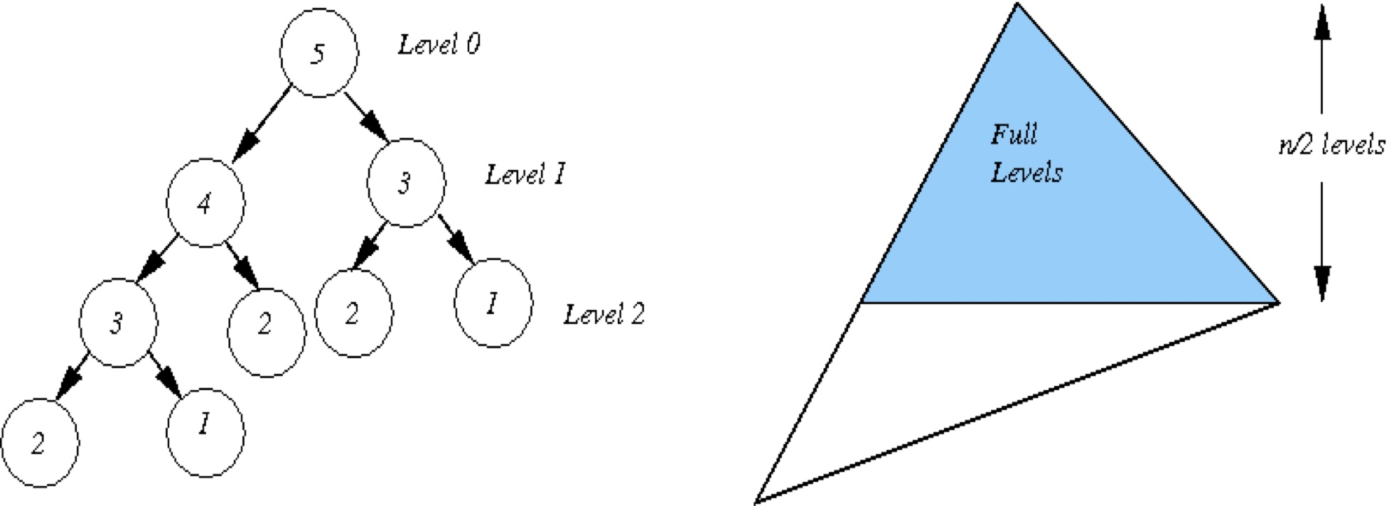
The reason why the above naive version is so ridiculously slow is repeated calculation. To do fib(5), you first call fib(4), which in turn solves fib(3) in the process. But then you need to call fib(3) again to combine with fib(4)’s result to form fib(5). In fact, everything except the leftmost branch is repeated:

The recursion tree is not a full perfect tree: the leftmost branch (with stepsize 1) has height \(n\) but the rightmost branch (with stepsize 2) has height \(n/2\). If you work out the math behind Fibonacci series, you will know the size of the tree is \(\sim 1.618^n\) which is related to the golden ratio, i.e., the time complexity is \(O(a^n)\) where \(a=\frac{\sqrt{5}+1}{2}\). See more details here: Fibonacci series approximates the golden ratio.

In fact, I plotted the runtime up to \(n=47\) below, which fits the curve \(y=c\cdot a^n\) very well for \(a=1.618\).

Memoized Recursion vs. Bottom-Up

But we all know that Fibonacci should be linear-time (modulo high-precision arithmetics), for example by a simple for loop (\(O(1)\) space):

def fib0(n):
  a, b = 1, 1
  for i in range(3, n+1):
    a, b = a+b, a
  return a

Note that the two assignments (=) above are simultaneous assignments (a nice feature of Python not found in C/C++/Java which would need auxiliary variables).

Or using a list to save all \(f(n)\)’s (\(O(n)\) space):

def fib1(n):
  f = [1, 1]
  for i in range(3, n+1):
    f.append(f[-1]+f[-2])
  return f[-1]

Both are bottom-up (from smaller \(n\) to larger \(n\)) and \(O(n)\) time. But the recursive version, though slow, does have its own merit: being top-down, it is identical to the original (recursive) definition, and is thus more “intuitive” from a mathematical point of view. How can we combine the merits of both approaches, i.e., a recursive function that runs in \(O(n)\) time?

The answer is memoization (note: not “memorization”), which means to remember the subproblems you already solved before and never solve the same subproblem twice. This technique is also known as tabularization, and thus needs a table that supports lookup, e.g., hash table (Python dict).

fibs={1:1, 2:1} # hash table (dict)
def fib2(n):
  if n not in fibs:
    fibs[n] = fib2(n-1) + fib2(n-2)
  return fibs[n]

These three versions fib1, fib2, and fib3 are all \(O(n)\) time, if we ignore the cost of high-precision arithmetics.

Caveat: you can see that the result of fib2(n) gets bigger and bigger exponentially, thus the cost of high-precision arithmetics should not be ignored for large \(n\). How many digits are there in \(f(n)\)? Well, we can just take the (say, base 10) logarithm on \(f(n)\), which we know grows \(\approx 1.618^n\) itself (actually the log base doesn’t matter in terms of complexity):

\[ \log f(n) \approx n \log 1.618 = O(n)\]

Thus each + operation would itself take \(O(n)\) instead of \(O(1)\) time! Therefore, fib2(n) actually runs in \(O(n^2)\) time for very large \(n\). Empirically, you can print the runtime to verify:

   n:    4096 base10-digits:    856 time:  0.000468
   n:    8192 base10-digits:   1712 time:  0.001572
   n:   16384 base10-digits:   3424 time:  0.005245
   n:   32768 base10-digits:   6848 time:  0.017311
   n:   65536 base10-digits:  13696 time:  0.063903
   n:  131072 base10-digits:  27393 time:  0.238554
   n:  262144 base10-digits:  54785 time:  0.929804
   n:  524288 base10-digits: 109570 time:  3.672851
   n: 1048576 base10-digits: 219140 time: 14.565167

As you can see, when n doubles, the number of digits in f(n) doubles, and the time quadruples.

Example 2: Number of Bitstrings

Now let’s look at our first non-Fibonacci example, number of bitstrings, and you will see that, although it does not look like Fibonacci at all on the surface, it can actually be reduced to Fibonacci.

Count \(g(n)\), the number of \(n\)-bit strings that do not contain "00" as a substring.

For example, for \(n=1\), both "0" and "1" are valid, so \(g(1)=2\), and for \(n=2\), among all 4 strings, 3 are valid (only "00" is not), so \(g(2)=3\).

What about \(g(0)\)? 0 or 1? It should be \(g(0)=1\) because the empty string "" is still valid!

How should we solve this problem? Still divide-n-conquer: we do a case analysis on the last bit (the \(n\)th bit), being either 1 or 0.

<==g(n-1)====>1  # last bit is 1
<==g(n-2)==>1 0  # last bit is 0, 2nd-last bit must be 1

• If the last bit is 1, then for the preceding \(n-1\) bits, every valid \((n-1)\)-bit string (there are \(g(n-1)\) of them) plus the last 1 bit makes a valid \(n\)-bit string;
• But if the last bit is 0, then we need to be a bit more careful because the second-last bit must be 1 otherwise we have 00. Now for the remaining \(n-2\) bits, every valid \((n-2)\)-bit string (there are \(g(n-2)\) of them) plus the last two bits (10) makes a valid \(n\)-bit string.
• Combining the two cases, we have \[ g(n) = g(n-1) + g(n-2). \]

Isn’t this exactly the same as Fibonacci?!

Well, don’t forget the base cases:

\[ g(0) = 1, g(1) = 2 \]

So this \(g(n)\) series is Fibonacci shifted by one step, i.e., \(g(n)=f(n+1)\).

Example 3: Maximum Weighted Independent Set on Linear Chain

Now let’s look at a more “real” example of DP, but in the end we’ll still reduce it to Fibonacci.

Given \(n\) numbers \(a_1, \ldots, a_n\), find a subset whose sum is the largest, with the constraint that no two consecutive numbers are chosen (i.e., if \(a_i\) is chosen, then neither \(a_{i-1}\) or \(a_{i+1}\) can be chosen).

For example, given

\[a=[9, 10, 8, 5, 2, 4]\]

the best solution is \([9, 8, 4] \rightarrow 21\).

Another way of presenting the problem is graph-theoretic one: given a linear-chain undirected graph:

9---10---8---5---2---4

you need to find the independent set that has the maximum sum value. An independent set of a graph is a subset of nodes where there is no edge between any two nodes. For linear-chain graphs, this is equivalent to “no two nodes in a roll”.

Greedy vs. Brute Force

You might come up with a very simple greedy strategy: always take the largest available number (let’s say \(a_i\)), cross out its two neighbors (\(a_{i-1}\) and \(a_{i+1}\)), and repeat until there is nothing left. Unfortunately, this is suboptimal; for example, for the above array, you’ll take \([10, 5, 4] \rightarrow 19\).

Instead, we can try exhaustive search, by enumerating all possible \(2^n\) subsets and evaluate all independent ones (i.e., those without two numbers in a roll). This is, however, too naive. A slightly better method is to write a recursion like Fibonacci. Given an array a of length \(n\), we ask the same question from the bitstrings problem: do you want to take the last number a[-1]?

• if you take it, then you should skip the previous number and solve the subproblem on the first \(n-2\) numbers, i.e., a[:-2];
• if you don’t take it, then you solve the subproblem of the first \(n-1\) numbers, i.e., a[:-1];
• a priori, you don’t know which choice is better (otherwise you’re greedy!), so you wait until the recursions report back their values (adding a[-1] to the first), and return the better one to your parent.

def mis0(a):
    if a == []: return 0 # empty
    if len(a) == 1: return max(0, a[0]) # singleton: only take if >0
    return max(a[-1] + mis0(a[:-2]), mis0(a[:-1]))

Of course, you must have noticed that doing list slicing costs \(O(n)\) time, so you would rather use an index i:

def mis1(a):
    def _mis(i):
        if i == -1: return 0 # empty
        if i == 0: return max(0, a[0]) # singleton
        return max(a[i] + _mis(i-2), _mis(i-1))
    return _mis(len(a)-1)

The singleton case is still rather ugly; a much cleaner version would be:

def mis2(a):
    def _mis(i):
        if i < 0: return 0 # empty
        return max(a[i] + _mis(i-2), _mis(i-1))
    return _mis(len(a)-1)

This version doesn’t need to deal with the singleton as a special case. When i==0, we can still either take a[0] and call _mis(-2), or not take a[0] and call _mis(-1); the max(0, a[0]) is thus automatically taken care of.

How fast would this version be? Well, same as naive Fibonacci!

DP

So how to make it much faster by DP?

Yes, you must have shouted, just memoization!

By now, you must have also realized that the constraint “no two numbers in a roll” is the exactly same as “no 00 as substring” with each 0 meaning “take this number”.

So we first define the subproblem:

Let \(f[i]\) be the best MIS value for the first \(i\) numbers, \(a_0, \ldots, a_{i-1}\).

The DP recurrence is simply:

\[f[i] = \max\{f[i-1],\quad f[i-2] + a_i\}\]

This is almost identical to the bitstrings problem, except we use \(\max\) instead of \(+\) between the two cases.

What about the base cases? We already discussed them in the brute force version:

\[ f[-1] = f[-2] = 0\]

(or \(f(i)=0\) for all \(i<0\), i.e., no numbers)

Here is an example (you can complete this table either bottom-up or top-down):

So we’ve got the correct answer of \(21\). However, this is only half of the problem. In optimization problems like this, we also need to return the optimal solution \([9, 8, 4]\) in addition to the best value of \(21\). This will be the topic of the next subsection.

DP is divide-n-conquer with multiple divides; combine and summary operators

After so much preparation, now we are finally ready to reveal the top secret of DP. In most textbooks, DP is described as “divide-n-conquer with memoization” or “divide-n-conquer with overlapping subproblems”. While these interpretations are correct and helpful, they do not answer the fundamental questions:

• What’s the key difference between divide-n-conquer and DP?
• What’s the reason for the “overlapping” subproblems?

The answer to them is:

• divide-n-conquer is a single divide with non-overlapping subproblems (think mergesort or quicksort)
• DP is divide-n-conquer with multiple divides,
  • which causes overlapping subproblems from different divides;
  • each divide alone still has non-overlapping subproblems, and after the recursive conquer steps and the combine step, one possible solution is formed;
  • among different divides, there is a new “summary” operator \(\oplus\) that “summarizes” the different solutions

There are thus two operators in DP:

• the old combine operator \(\otimes\) from divide-n-conquer, such as the concatenation operator in quicksort, or the mergesorted function in mergesort; in MIS, it is + (+a[i] or +0) while in Fibonacci/bitstrings it is * (*1).
• the new summary operator \(\oplus\) such as + in Fibonacci/bitstrings and max in MIS.

Therefore, in the three problems we have seen so far, the \(f(n-1)\) and \(f(n-2)\) are not two subproblems, but rather two different divides with each divide being a unary one like quicksort/quickselect worst-case (\(T(n)=T(n-1)+...\)). These unary divides also happen to be “incremental” ones, as they always reduce problem size by 1 or 2, rather than split it by half as in binary divides. If you understand this paragraph, your level of DP is already above 99.9% of computer science students!

You might be rightfully asking, why all unary divides? Are there binary divides in DP like mergesort or quicksort best-case? The answer is certainly yes, which we will discuss in the next section; but they’re a bit more advanced than unary divides so many textbooks skip them (or only discuss them superficially).

What I presented above is the “semiring” view of dynamic programming; semiring is a concept in abstract algebra, which is much more advanced than linear algebra and the foundation of modern mathematics. While this algebraic view might be a bit too advanced (never appearing in a standard textbook), I hope you can more or less understand this key idea, which will greatly improve your level of understanding of DP.

Historical Notes

The term “dynamic programming” was coined by Richard Bellman at RAND in 1955 who began the formal study of DP (and is now remembered as the inventor of DP), although elements of DP were known before. Specialized forms of DP have been reinvented numerous times; the most well-known of these was the Viterbi algorithm. The funny thing is that Andrew Viterbi and Richard Bellman were colleagues at UCLA (in different departments though), and yet Viterbi didn’t know that Bellman had already invented a much more general form of DP many years ago. Viterbi “reinvented” the (restricted subclass of) wheels, but generalizations of his algorithm became so widely used in signal processing, information theory, language and speech processing, computational biology, etc., that people often view many DP algorithms as instances of Viterbi in those fields, which is totally the opposite of historical development! For example, in natural language processing (NLP), the word “Viterbi” even became a widely used adjective meaning “best”; in NLP papers, people often say things like “Viterbi tree” or “Viterbi alignment”. The take-away message is that (1) nothing is new under the sun, (2) important things always get reinvented many times, (3) the more important a thing is, the more times it is reinvented, and (4) therefore don’t get depressed if you’re scooped (I got scooped many many times in my career) – if anything, it only means that you’ve (re-)invented something important!

We will discuss the Viterbi algorithm in the graph chapter.

The semiring view of DP dates back to … semiring parsing…