\(\renewcommand{\vec}[1]{\mathbf{#1}}\)
\(\newcommand{\vecw}{\vec{w}}\) \(\newcommand{\vecx}{\vec{x}}\) \(\newcommand{\vecu}{\vec{u}}\) \(\newcommand{\veca}{\vec{a}}\) \(\newcommand{\vecb}{\vec{b}}\)
\(\newcommand{\vecwi}{\vecw^{(i)}}\) \(\newcommand{\vecwip}{\vecw^{(i+1)}}\) \(\newcommand{\vecwim}{\vecw^{(i-1)}}\) \(\newcommand{\norm}[1]{\lVert #1 \rVert}\)
In this Exploration, we will explain some of the most important and useful concepts in machine learning.
First, let us define the three types of datasets and the corresponding errors.
Training set and training error: Each machine learning algorithm is trained on a “training set” of labeled examples, \(D = \{(\vecx^{(i)}, y^{(i)}) \mid i = 1 \ldots |D|\}\). In this set, each example \(\vecx^{(i)}\) comes with a label \(y^{(i)}\); for example, if you want to train a handwritten digit classifier, you can collect, say, 1,000 handwritten digit images, and each image has a groundtruth label from the set {0, 1, …, 9}. Your training algorithm aims to minimize the error on this training set, which we call the “training error”.
Test set and test error: But actually, the training error is not the most important metric we care about in practice. Instead, we care much more about the performance of your trained model on previously unseen examples, i.e., error at testing time. This set of previously unseen examples is called the “test set”, and the error on it is called the “test error”. This is analogous to our own learning as a student: the training set is like the textbook, and the test set is like the exam. While we might want to be as familiar as possible with the textbook, it is NOT the ultimate goal of learning. A student who memorizes the whole textbook may or may not do well on exams with unseen questions. Similarly, we do NOT want our machine learning model to memorize the whole training set; we want it to “generalize” to previously unseen examples that are similar to the training ones. So “test error” is the main metric we use to evaluate machine learning models and algorithms.
Generalization error: A highly related, but more theoretical and abstract, concept is the “generalization error”, which is defined as the “expected” test error, over the distribution of all possible test sets. In machine learning theory, this error is what we want to minimize. But in practice, this generalization error is often estimated by the test error on a test set because the true distribution of all possible test sets is hard to categorize.
Three subtypes of test sets:
“non-blind” test set: In most research papers, we often divide the labeled data set into training and test tests. In this case, the test case is not blind since you know the groundtruth labels for all test examples. Therefore, the person who trains the model (the “trainer”) can evaluate and report the test error him/herself. However, this also means that in theory s/he can “cheat” on this kind of test set, or only report the model that does best on this test set, which we will see later is an instance of overfitting.
“semi-blind” test set: A slightly better test set is a semi-blind one, where the test set contains unlabeled examples (i.e., only \(\vecx\) but no corresponding \(y\)), so it is much harder (but still possible) to cheat. The trainer needs to submit to the grader the predicted labels of the test examples. Our homework assignments mostly use semi-blind test sets.
“blind” test set: The best test set is truly blind, in the sense that the trainer does not even have access to the test examples, not to mention the labels. In this case, the trainer needs to submit the model itself (rather than the test predictions) to the grader, who runs it on a hidden test set. Some online competitions like SQuAD question answering use blind test sets.
Dev set and dev error: To simulate a real test set (which we can not predict), a standard practice is to held out a small portion (say, 5-10%) of the training set as the “development set”, or “dev set” for short. We do not train on this dev set, but rather use it to monitor the model’s performance on unseen data during the training process (using the “dev error”), and to prevent the phenomenon of “overfitting” which we will discuss next.
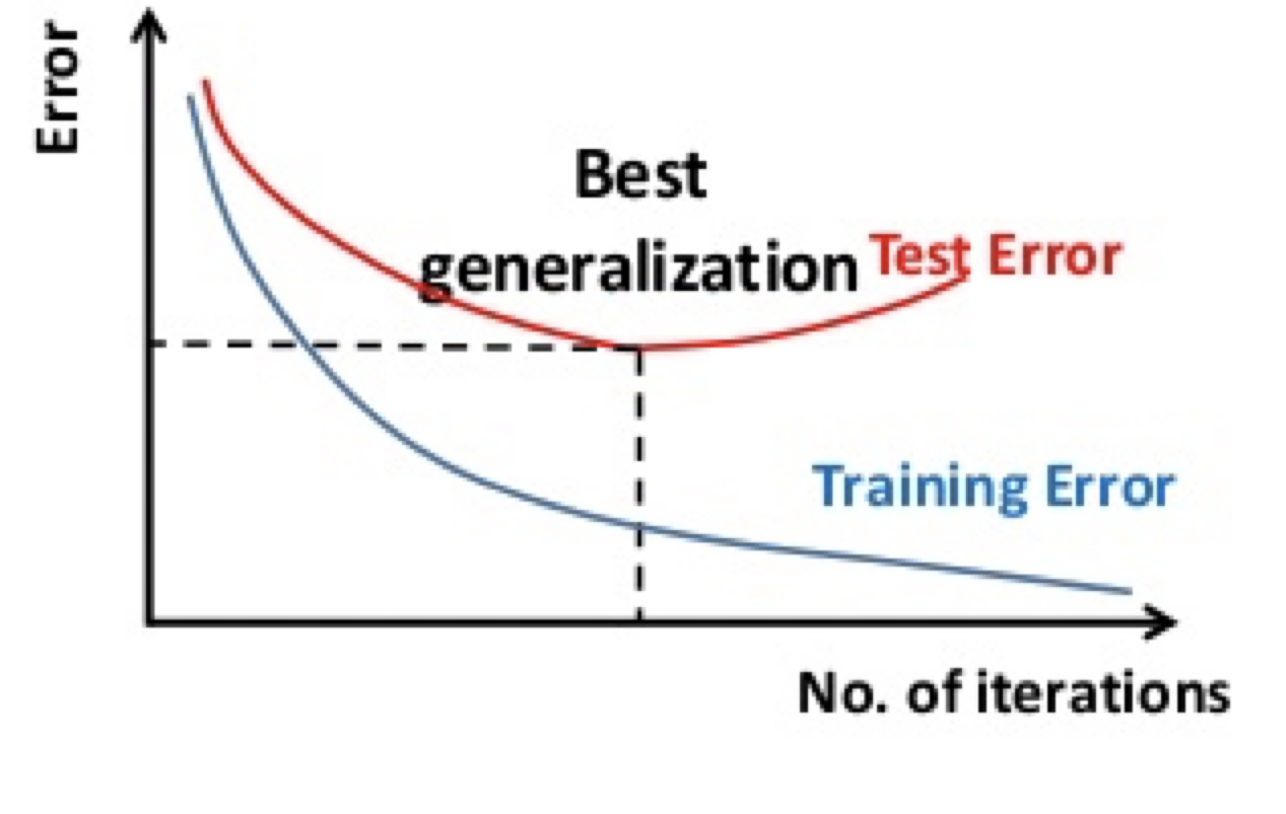
As mentioned above, ultimately we care about the test error, not the training error. As training progresses (e.g., over more and more training data, or using larger and larger models), we will see the training error keeps decreasing. However, the test error (e.g., simulated by the dev error) first decreases but then after a certain point, starts to increase.

This phenomenon is called “overfitting” which means the model is starting to memorize the idiosyncracies (such as outliers or noise) of the training set, rather than learning something fundamental about the prediction task. Overfitting is the single most common pitfall in machine learning.
Overfitting occurs not only due to overtraining, but also due to excessive model capacity. For example, in this curve fitting example, if data has some noise, and if you use a very high degree polynomial to fit the data, it will fit very well (in the extreme case, with zero training error). But this high-degree polynomial is definitely unlikely to capture the real distribution behind the training data, and is unlikely to generalize well.

On the opposite end, if the model capacity is too small or training is insufficient (e.g., too few iterations), we will see “underfitting”. But generally speaking, this problem is not as severe as overfitting.
There are three common ways to prevent overfitting:

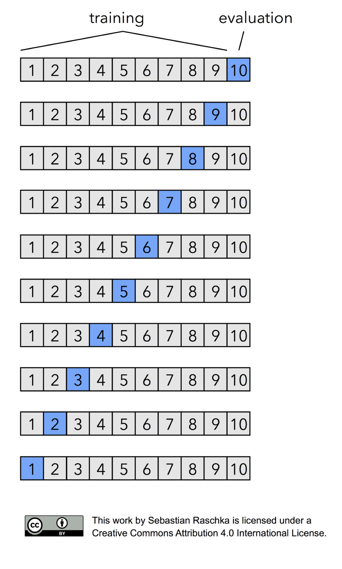
While it is common to set out a small portion of the training data as dev set, one might wonder what if that portion is not very representative of the whole set. It would certainly be better to try every portion as a dev set, so this is what is known as “leave-one-out cross-validation”. We divide the data into, say, \(N=10\) subsets, and train on the first 9 subsets and test on the last subset, and then train on subsets 1,2,…,8 and 10 and test on subset 9, and so on. In other words, we always leave out one subset and train on the remaining \(N-1\) subsets. As \(N\) increases, this cross-validation error is the best approximation of the generalization error based on the data we have (assuming the training and test data sets follow the same distribution).
