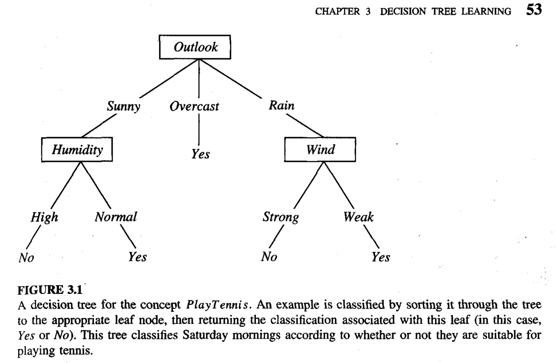
A decision tree is a set of decisions made according to the input features of a given data point organized in a hierarchical structure (a “tree”). A decision tree might look something like this:
(The above image is sourced from figure 3.1 of Tom Mitchell’s textbook, “Machine Learning”).
The boxes labeled with input features (e.g., “Wind”, “Outlook”, etc) in the above diagram are referred to as nodes. The nodes are connected by edges, each labeled with a value (e.g., “Sunny”). The top node is specifically referred to as the root node. The Yes’s and No’s are also nodes; they’re specifically referred to as leaf nodes. A leaf node is any node that doesn’t have more nodes connected to it via edges from below (i.e., leaf nodes have no “children”).
When a data point is processed by the decision tree, its input features are analyzed by the decision nodes (non-leaf nodes) in the tree one at a time, starting at the root (the top of the tree) and working down toward a leaf. Each leaf node is associated with a certain final answer for the predicted output.
In the above diagram, the goal of the decision tree is to determine whether it’s a good day to play tennis. Hence, the decision nodes (the non-leaf nodes) analyze input features about the weather (outlook, humidity, wind, etc), and the leaf nodes each correspond to either a “Yes” or “No” answer (“Yes”, it’s a good day to play tennis, or “No”, it’s not).
Suppose that the outlook for today’s weather is sunny, the humidity is normal, and the wind is strong. We want to determine whether it’s a good day to play tennis, so we refer to the above decision tree diagram. Again, decision tree processing always starts from the root node, so we first analyze the weather’s outlook. The outlook is sunny, so we follow the left edge down to the “humidity” node. This node analyzes the humidity. The humidity is normal, so we follow its right edge down to a “Yes” leaf node. Since this is a leaf node, it provides a final answer for the predicted output: “Yes”, the decision tree predicts that today will be a good day to play tennis.
In this case, the wind was irrelevant to the prediction. Indeed, a given path down a decision tree from the root to a leaf will not necessarily analyze every input feature.
Decision trees were traditionally (and often still are) crafted manually by experts in a given domain. But it’s also possible to use machine learning techniques to build a decision tree automatically such that it achieves good performance (e.g., high accuracy) on a given training set.
Decision trees can be used for both classification and regression tasks, but we’ll just focus on decision trees for classification (as in the previous diagram—classifying a day as either good or bad for tennis-playing, given the weather).
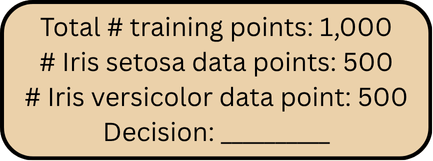
Let’s use a different example, though. Suppose the goal is to classify the species of an iris flower based on measurements of its petals and sepals. Perhaps the training set has 1,000 data points, 500 of which belong to the species Iris setosa and the other 500 of which belong to the species Iris versicolor.
To build a decision tree classifier for this task, we first create a root node; decision trees are always grown top-down, so we always start with the root. We then place all the data points from the entire training set “inside” the root node:
The tree is then grown downward incrementally. First, the data in the
root node (i.e., all the training data) is split into groups (usually
two groups) according to a decision. Each decision is typically given by
an input feature and a threshold. For example, the decision could be
something like petal_length < 2 (the input feature is
petal length, and the threshold is 2mm). In such a case, all of the data
points in the root node are split into two smaller groups: 1) a group
consisting of all the data points from the root node with petal length
less than 2mm, and 2) a group consisting of all the data points from the
root node with petal length greater than or equal to 2mm.
These two groups are then placed into their own respective nodes immediately below and connected to the node from which they were split (the root node, in this case).
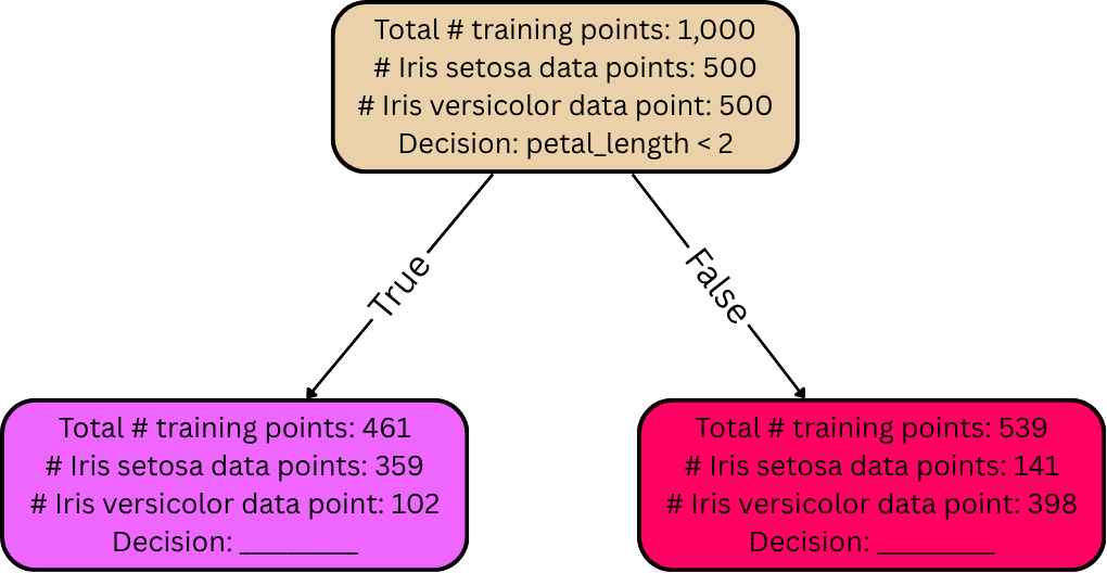
The “True” edge on the left corresponds to training data whose petal length is, indeed, less than 2mm. The “False” edge on the right corresponds to training data whose petal length is not less than 2mm (i.e., whose petal length is greater than or equal to 2mm). The split-off child nodes are colored to visually depict the separation of labels. Nodes containing more Iris setosa training data points are colored more blue, and nodes containing more Iris versicolor training data points are colored more red.
But how did we select the decision petal_length < 2?
Well, when building a decision tree for classification, decisions are
usually selected to minimize the “diversity” of labels in the split-off
nodes (this diversity can be measured in various ways). For example, the
root node in this case is extremely diverse—a perfect 50/50 mix between
the two flower species. When a decision is selected to split the data
into two smaller groups, the goal is to get all of the Iris
setosa data points into one group, and all of the Iris
versicolor data points into the other group—two split-off groups of
data that each have no diversity in their labels whatsoever.
Of course, this goal likely isn’t possible in practice; regardless of
the selected input feature and threshold, it’s likely impossible to
cleanly split the data into two “pure” groups with no diversity
whatsoever. However, if the decision is selected carefully, the
average diversity of the two groups can still be reduced
relative to that of the node from which they were split (the root node,
in this case). For example, in the above diagram, the root node was a
50/50 mix of the two flower species, but the two split-off nodes
achieved much lower diversity than that. The left node contains mostly
Iris setosa training data points, and the right node contains
mostly Iris versicolor training data points. The objective of
the splitting process is to select the decision (input feature and
corresponding threshold) that splits the data into two new groups with
the lowest possible average diversity. In this case, the input feature
petal_length and threshold \(2\) were selected as the decision that
accomplishes that objective.
Note: The diversity of labels of the data in a node can be measured in various ways. The two most common measures are entropy (information gain) and Gini impurity. Regardless of which measure is used, the goal is usually to select decisions that minimize its average value across the two newly split-off groups of data.
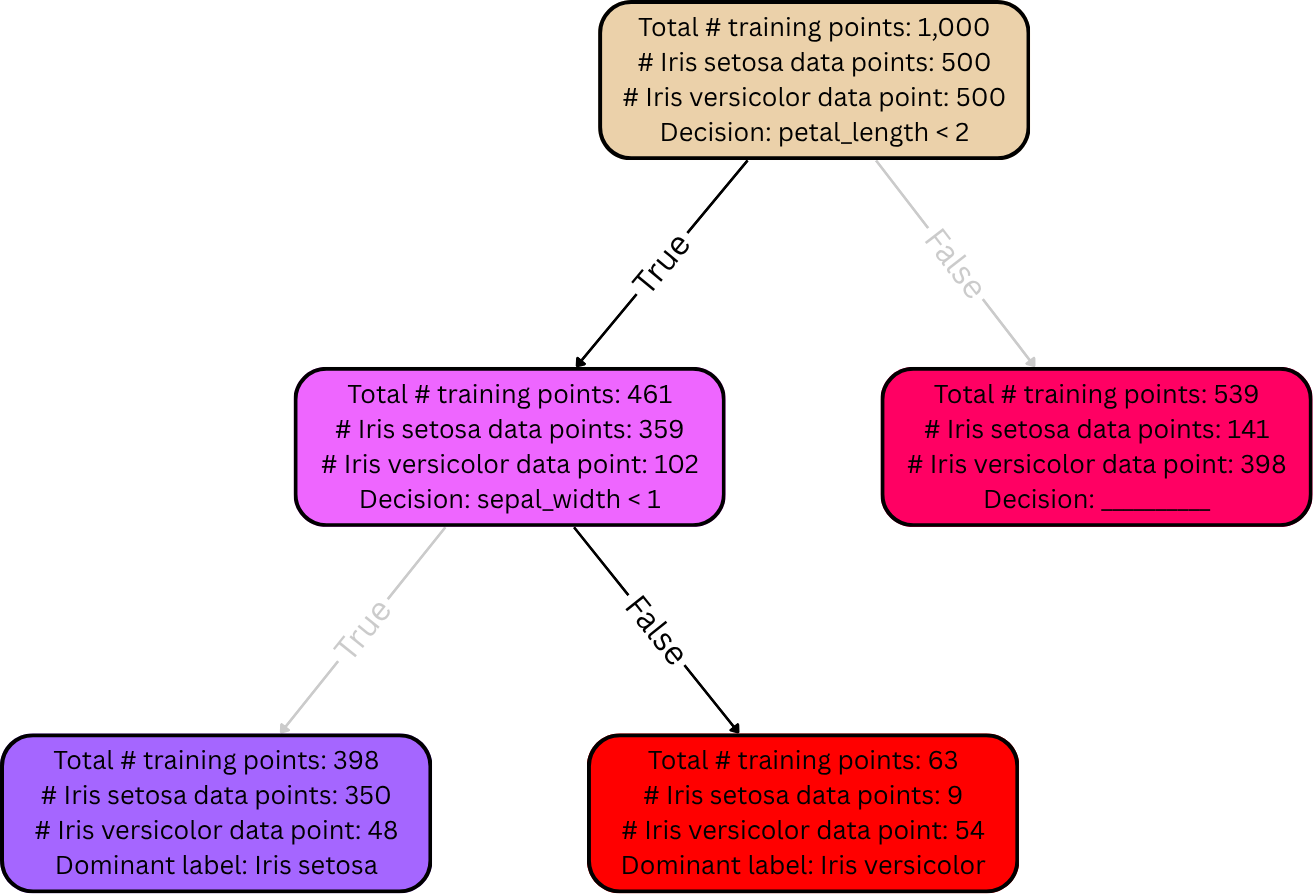
From here, the tree is split even further: the data in those two split-off nodes’ groups are each be split again into even smaller groups according to new decisions, producing child nodes that are even less diverse. Here’s a depiction of one of those subsequent splits:
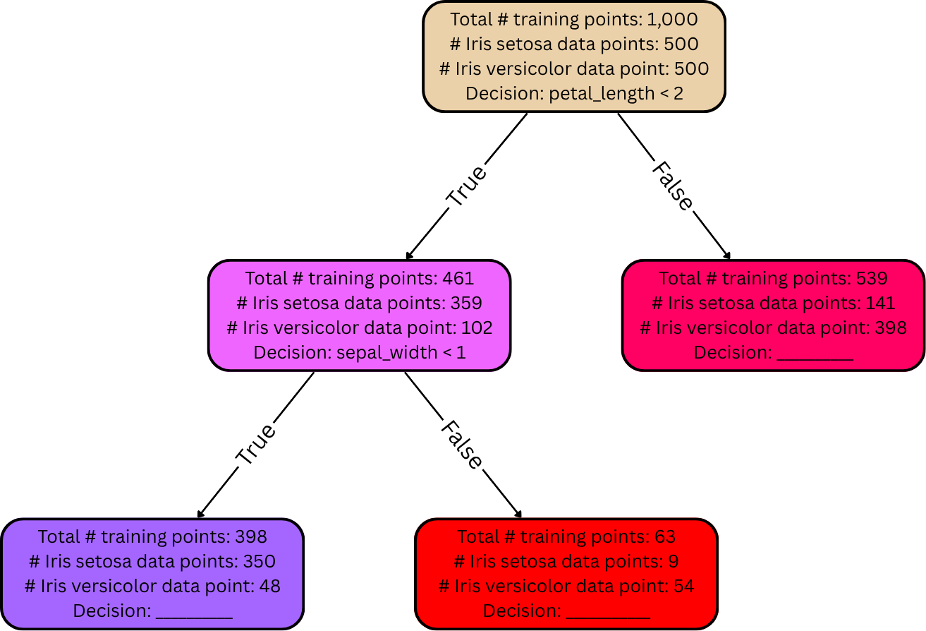
Notice: nodes that are further down the tree tend to be more “pure” / less diverse. In the simplest case, this splitting process continues until all the leaf nodes in the tree are completely pure, meaning for each leaf node in the entire tree, all training data belonging to its group have the same label (zero diversity). In practice, though, the splitting process is often terminated early, so the leaf nodes typically aren’t completely pure. We’ll discuss this more momentarily.
After the decision tree is fully grown, it can be used to make predictions (e.g., on a dev set or a test set). As explained earlier, each leaf node is supposed to represent a certain final answer for the predicted output. The rule here is simple: if, when analyzing a data point, it falls into a certain leaf node, its label is predicted to be whichever label is most frequent among the training data in that same leaf node. For example, suppose that a given flower has petal length 1.5mm and sepal width 2mm. Then applying the decision tree from the diagram in the previous section, it would take the left (“True”) edge down from the root node because its petal length is less than 2, and then it’d take the right (“False”) edge down from there because its sepal width is greater than 1mm. Suppose there are no more decisions / edges from there. Then it has landed in a leaf node. This particular leaf node has 9 training points belonging to the Iris setosa species, but 54 belonging to the Iris versicolor species. Since most of the training points in this leaf node belong to Iris versicolor, the decision tree predicts the given flower’s species to be Iris versicolor accordingly.
(i.e., if a flower lands in a red-colored leaf node, then the decision tree predicts its species to be Iris versicolor; if it lands in a blue-colored leaf node, then the decision tree predicts its species to be Iris setosa).
If a decision tree is allowed to keep growing until every leaf node is completely pure, its final leaf nodes will often be very small (i.e., each will have very few training data points in it), and overfitting may ensue. In fact, any such decision tree will always achieve perfect accuracy on the training set (unless there are data points with identical input features but different labels), but they’ll often achieve poor accuracy on data outside the training set (e.g., on a dev set, or a test set).
A common solution to this problem is to stop splitting nodes earlier in the process, limiting the size of the tree. For example, a max depth might be specified, and the splitting process will be stopped early so as to prevent any leaf nodes from exceeding that depth (the depth of a node is a measure of how far away it is from the root). The value of the max depth might be chosen so as to maximize performance on a held-out dev set.
Such strategies produce smaller, simpler decision trees, and their leaves tend to have more training points inside them. This reduces overfitting issues, but it can introduce underfitting issues—some of the leaf nodes might not be fully pure (because the splitting process stopped early), meaning that at least some training points are going to fall into a leaf node that predicts their label incorrectly. For instance, in the diagrams from the previous examples, there were 9 training points belonging to the Iris setosa species that landed in a red-colored leaf node at the bottom (i.e., a leaf node that contained mostly training points belonging to the Iris versicolor species). Those 9 training points were the minority in their leaf node. If the decision tree were to be used to classify any one of those 9 training points, it’d incorrectly predict the label to be Iris versicolor.