The perceptron algorithm was invented around 1959 by Cornell psychologist Frank Rosenblatt (1928-1971), a pioneer of the field artificial intelligence. As we will see in this module, the vanilla perceptron is basically a single neuron, and multilayer perceptron is the foundation of today’s deep learning. Therefore, Rosenblatt is sometimes called the father of deep learning, and his work on perceptron was ~60 years ahead of time.
However, the research on perceptron came to a halt around 1969 (First AI Winter) due to inability to solve inseparable cases, and it was not until 30 years later in 1999 that perceptron was revived, with the new form of large-margin classifiers, voted and averaged perceptron (Freund and Shapiro, 1999). Starting from 2012, the multilayer version of the perceptron is widely used in the deep learning revolution that has deeply impacted our daily lives.
One of the simplest yet still one of the most powerful models in classification is linear classification. What do we mean by “linear classification”? Well, we mean that the model is a linear model, i.e., its decision is based on the linear combination of input features. For example, let us consider a (very crude) toy example: classifying a person based on two features, age (\(a\)) and number of working hours per week (\(t\)), into two classes, i.e., whether this person earns 50K or more annually. The intuition is that a person with more experience (age) and more working hours tend to earn more. Apparently this would not be very accuate at all, but it serves our purpose of illustration. The linear model just looks at a linear combination (i.e., weighted sum) of these two features, and check whether that weighted sum exceeds a threshold (if it does, we output YES otherwise NO):
\[ w_1 \cdot a + w_2 \cdot t > \theta\]
Here weights \(w_1\) and \(w_2\) and the threshold \(\theta\) are the three parameters to be learned from the training data, which contains many example persons, each with an age and a number of hours, plus the label YES/NO. The goal of the machine learning algorithm is to tune or fit these parameters to perform well on the training set. For example, if in a training set, age is much more important than the number of hours, then you would expect the weight \(w_1\) to be higher after training.
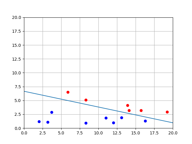
Geometrically, the above equation is basically drawing a line, or “decision boundary” on the 2D coordinate space where the x-axis is age and y-axis is hours. Every point top-right of that line would be classified positive, and every point lower-left of that line would be classified negative.
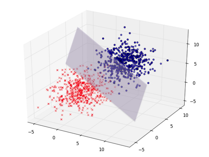
More generally, if you have many many other features, such as gender, race, country-of-original, educational-level, marriage-status, job-sector, etc., you will in a high-dimensional space of \(n\) dimensions (\(n\) being the number of features). Now the decision boundary is not a line, but a hyperplane, called “separating hyperplane”, that still divides this high-dimensional space into two halves, one positive and one negative. This hyperplane has dimensionality \(n-1\) (e.g., a line in 2D space, a plane in 3D space).
In \(n\) dimensions, we represent each data point by a \(n\)-dimensional vector \(\mathbf{x}=(x_1, x_2, \ldots, x_n)\), and we represent a decision boundary by a weight vector \(\mathbf{w} = (w_1, w_2, \ldots, w_n)\); this weight vector is orthogonoal to the decision boundary (thus also called a “norm vector”) and points to the “positive” side. In other words, for any data point \(\mathbf{x}\), if it more-or-less agrees with the direction of the weight vector \(\mathbf{w}\), then it is classified as positive, otherwise negative. Mathematically, the “agrees in direction” is measured by the project of \(\mathbf{x}\) onto \(\mathbf{w}\), calculated by the dot product
\[\mathbf{x} \cdot \mathbf{w} = x_1 w_1 + x_2 w_2 + \ldots + x_n w_n\]
If this dot product is positive, we classify this \(\mathbf{x}\) as positive, and negative if otherwise.
Now we are given a training set \(D = \{(\mathbf{x}^{(i)}, y^{(i)}) \mid i = 1 \ldots |D|\}\) which is a set of training examples \(\mathbf{x}\) and their corresponding labels \(y \in \{+1,-1\}\), and want to fit a weight vector \(\mathbf{w}\) so that it can correctly classify all training examples. This means at the end of training, for each training positive example \((\mathbf{x}, +1) \in D\), we would have a positive dot product \(\mathbf{w} \cdot \mathbf{x} > 0\) and for each negative example \((\mathbf{x}, -1) \in D\), we would have a negative dot product \(\mathbf{w} \cdot \mathbf{x} < 0\). These two cases can be combined in one formula:
\[y (\mathbf{w} \cdot \mathbf{x}) > 0\]
If such a weight vector is found during training, we say the perceptron algorithm has “converged”.
The training procedure of the perceptron algorithm is extremely simple and intuitive (much like human learning). It could be summarized by the following steps:
initialize weight vector \(\mathbf{w}\)
cycle through the training data (multiple iterations)
until all examples are classified correctly
First, we initialize the weight vector \(\mathbf{w}\) to be the zero vector \(\mathbf{0}\) (in \(n\) dimensions), i.e.,
\[\mathbf{w} \gets (0, 0, \ldots, 0)\]
Note that according to the decision rule, this initial weight vector would output negative on all examples since the dot product is always \(0\) and we said we output positive if the dot product is positive and negative if otherwise.
Then we try to improve this weight vector by trial-and-error. Baiscally, we cycle through the training set until convergence (i.e., performing multiple iterations over the whole training data) and make updates to \(\mathbf{w}\). In each iteration, for each training example \((\mathbf{x}, y) \in D\), we try to use the current weight vector to classify it. If the result is different from the correct label \(y\), i.e., the example \(\mathbf{x}\) is positive (\(y=+1\)) but \(\mathbf{w}\cdot \mathbf{x} < 0\) thus outputing negative, or vice versa, we call it a mistake. More formally, a mistake happens when
\[ y \cdot (\mathbf{w}\cdot\mathbf{x}) \leq 0\]
Notice that the tie-breaking case, \(\mathbf{w}\cdot\mathbf{x} = 0\), i.e., when \(\mathbf{x}\) lies exactly on the decision boundary, is also considered a mistake, because we want our model to be strictly correct on each example, not by chance. In other words, the initial zero weight vector would cause a mistake on any training example regardless of the label.
When a mistake happens, we need to improve the weight vector by an update using the mistaken training example. For instance, for a positive example \(\mathbf{x}\) with \(y=+1\), we would hope \(\mathbf{w}\cdot\mathbf{x} > 0\) but the dot product is currently negative or zero. How would we make the dot product more likely to be positive (or at least less negative)? We would add \(\mathbf{x}\) to \(\mathbf{w}\):
\[ \mathbf{w}' \gets \mathbf{w} + \mathbf{x}\]
This way the new dot product is always larger (more positive or less negative) than the original dot product:
\[ \mathbf{w}' \cdot \mathbf{x} = \mathbf{w}\cdot\mathbf{x} + \mathbf{x}\cdot\mathbf{x} > \mathbf{w}\cdot\mathbf{x}\]
because the self dot product \(\mathbf{x}\cdot\mathbf{x} = |\mathbf{x}|^2\) is always positive.
Here is an example update on a positive example. 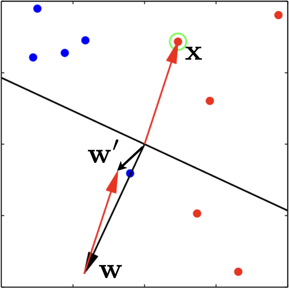
Note, however, that after the update, we are not guaranteed to be correct on this example. The only thing we can be sure is that we will be less wrong on it. For example, in the above figure, example \(\mathbf{x}\) is positive (all green dots are positive), and the current weight vector \(\mathbf{w}\) points to the opposite direction which causes the dot product to be negative. After we apply the update, the new weight vector \(\mathbf{w}'\) is still wrong on this example, but much more aligned with it, i.e., much less wrong. In case in the next iteration over the training data, this example is incorrect again, we will apply another update, and eventually it will be correct.
Similarly, for a mistake on a negative example \(\mathbf{x}\) with \(y=-1\), we subtract \(\mathbf{x}\) from \(\mathbf{w}\):
\[ \mathbf{w}' \gets \mathbf{w} - \mathbf{x}\]
so that the new dot product is smaller (more negative or less positive).
We can unify the two update cases as:
\[ \mathbf{w}' \gets \mathbf{w} + y \cdot \mathbf{x}\]
We cycle through the whole training set multiple times, and if in one round, all examples are classified correctly by the weight vector (thus no update at all), we say the perceptron algorithm has converged.
Luckily, we have a powerful theorem that states that if the data is separable (i.e., there exists a hyperline that separates positive and negative examples, or equivalently, there exists some weight vector that can correctly classify all examples), then the perceptron algorithm is guaranteed to converge after finite number of mistakes (i.e., updates).
In practice, however, we do not know a priori if our training data is separable, and even if it is, we do not want to train until convergence because it might be overfitting. So we often use a dev set to monitor the training progress and pick the model that works the best on the dev set to prevent overfitting to the training set.
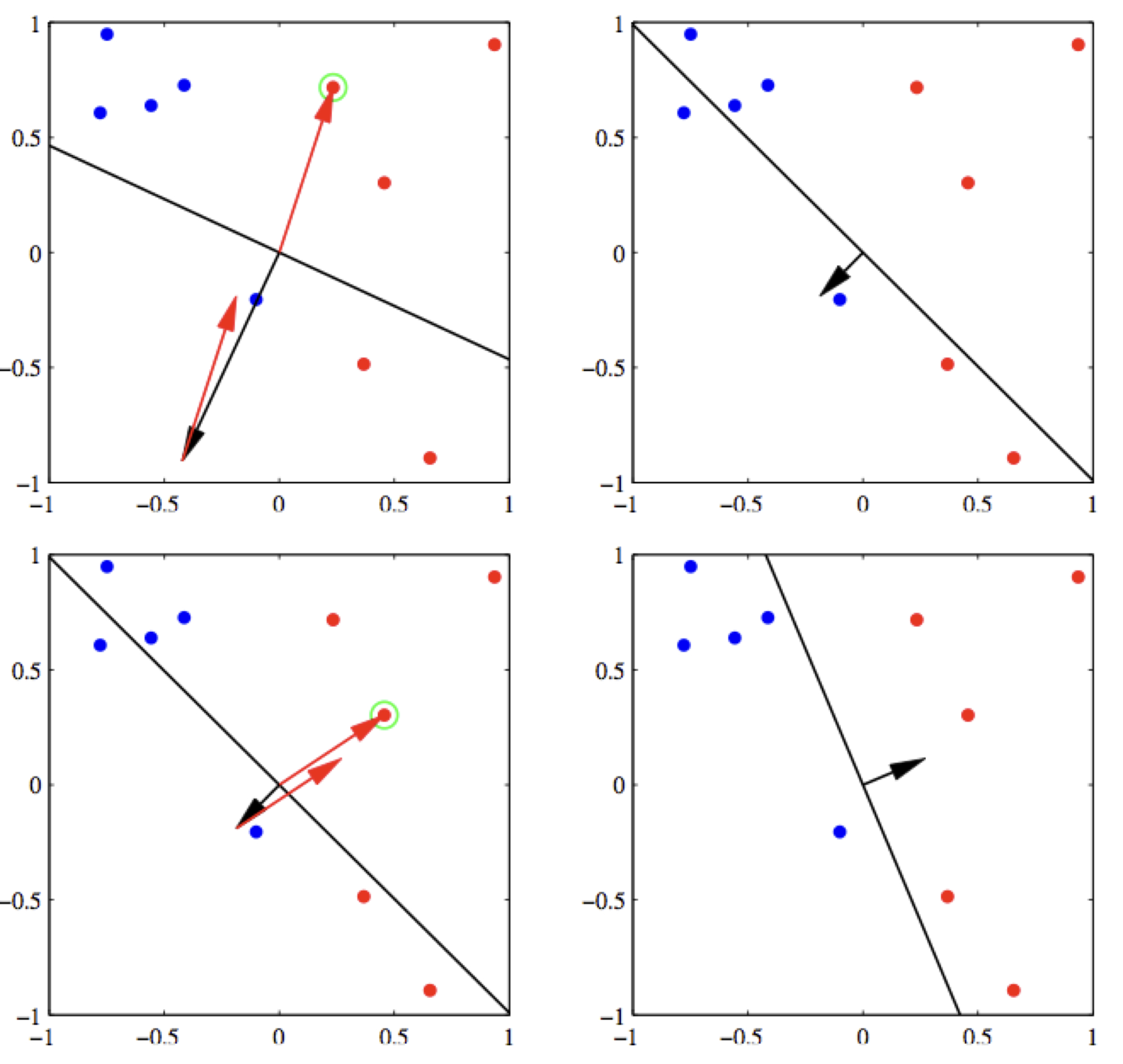
Here is a demo run of perceptron with two updates, and the final weight vector correctly classifies all examples.