(Source: Modified from ImageNet example images. Original image author(s) unknown.)

(Source: Wikimedia Commons. Autonomous-driving-Barcelona.jpg. Author: Eschenzweig. License: CC BY-SA.)
In this exploration, we’ll examine how deep learning revolutionized computer vision through Convolutional Neural Networks (CNNs). You’ll learn how images are represented as data, discover the breakthrough ImageNet competition that changed the field, and understand how CNNs use specialized layers to automatically detect visual patterns—from simple edges to complex objects.
Computer vision is a subfield of computer science that focuses on devising methods to process and analyze images and videos. Computer vision is a very broad subfield. Some common computer vision tasks include:
Other examples abound.
Many computer vision tasks have been around since long before the modern era of deep learning. Such tasks were historically solved using more “traditional” computer vision techniques. These techniques are often very efficient and are still occasionally used today for simple computer vision tasks (e.g., image stitching to generate panoramas). However, deep learning has enabled the creation of systems that can address much more complex computer vision tasks, like classification of complex images (e.g., species of animals, makes and models of cars, etc) and even image and video generation. Deep learning has also been applied to improve performance on many simpler tasks as well.
To understand how deep learning is used to tackle computer vision tasks, you first must understand how images are represented in these systems.
A pixel is essentially a very small colored square. A modern computer monitor or other device screen typically displays millions of pixels tightly packed into a grid. That is, in most typical representations, a digital image is simply a collection of tiny, colored squares. You can often see this if you zoom in on an image very closely:
![]()
Since each pixel in an image is simply a colored square, storing a pixel’s information (e.g., in a raw image file, or in a computer program’s memory) just requires recording its color. There are lots of ways that colors can be represented and stored in a computer, but a common format is RGB (red, green, blue). Basically, the color of a pixel is broken down into constituent red, green, and blue channels. Each channel is represented by a single number, often between 0 and 255.
For example, suppose a pixel’s numeric RGB sequence is 10, 14, 247. Then its red channel has value 10, its green channel has value 14, and its blue channel has value 247. This would represent a pixel that’s a very bright blue color—its blue channel has a much higher value than its red or green channels.
(For context, a completely white pixel has a numeric RGB sequence of 255, 255, 255, and a completely black pixel has a numeric RGB sequence of 0, 0, 0.)
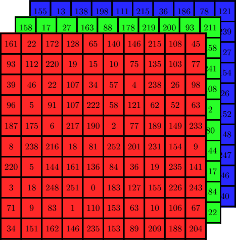
That’s all to say, an image can be represented as a grid of pixels, where each pixel is in turn represented as three numbers—one for each of the R/G/B color channels. Or, equivalently, an image can be represented as three grids of numbers: one to represent the red channel values of each pixel, one for the green channel values, and one for the blue channel values.
Grayscale (black-and-white) images are even simpler: for each pixel, rather than storing three numbers (one for each color channel), it’s possible to store only a single number representing the pixel’s brightness. Perhaps 0 represents black, 255 represents white, and everything in between represents varying shades of gray. This means that a grayscale image can be represented as a single grid of numbers (instead of three stacked together).
Lastly, these numbers don’t actually have to be between 0 and 255. That’s just how they’re often stored (e.g., in an image file). It’s very common for these numbers to be rescaled just before processing them for some computer vision task. For example, they might be rescaled to be between 0 and 1, or they might be standardized so that they have a mean of 0 and a standard deviation of 1 across a large dataset.
Since images can be represented as numbers, they can be provided as inputs to machine learning models, such as multilayer perceptrons (MLPs) from the previous section, which can then be trained to make predictions about them (e.g., classifying an image as either a dog or a cat).
To be clear, MLPs are not very good at computer vision tasks, at least when compared to other more structured neural network architectures (e.g., CNNs; more on these in a moment). But for simple tasks with sufficient training data, they can perform decently well. One famous benchmark is the MNIST database (Modified National Institute of Standards and Technology). It consists of a large set of 28x28 grayscale images of handwritten digits:

(Source: Wikimedia Commons. MNIST_dataset_example.png. Author: Suvanjanprasai. License: CC BY-SA.)
An MLP trained to classify MNIST images into their respective digit classes (i.e., to analyze these images of a handwritten digits and determine which digits they are) can achieve a classification accuracy of over 99% (see, e.g., Ciresan et al.).
However, as it turns out, classifying handwritten digits is fairly easy. Classifying arbitrary objects—dogs, cats, cars, trees, people, and so on—is much harder. And other computer vision tasks, like detecting and identifying individual objects in a complex scene, or generating realistic videos to match given text prompts, can be even harder. While MLPs perform fairly well on MNIST, they struggle with these more complicated computer vision tasks.
Plain-old MLPs aren’t really designed for computer vision tasks, though. For one, they’re not robust to small changes that commonly occur in image data. Suppose you take a picture of your dog and give it to an MLP, and the MLP correctly classifies it as a dog. But then suppose your dog takes a small step to the left. You then take another picture and give it to the MLP as well. This time, the MLP might make a wildly different prediction. It might predict it to be a cat, for example. This is because every pixel in a given image is treated as a separate input feature, and each input feature is multiplied by its own completely separate weights within the MLP. When the dog takes a step to the left, perhaps the pixels comprising the dog look the same as before, but they’re in a slightly different location in the image, corresponding to completely different input features that are multiplied by completely different weights. That’s to say, MLPs are extremely sensitive to small movements of objects (and / or movements of the camera). This issue often manifests as overfitting, and avoiding it might require an extremely large amount of training data.
As deep learning techniques advanced and became capable of solving more complex computer vision tasks, it became apparent that we needed more data—bigger datasets on which to train these deep learning models, and more complex tasks against which to test them so that we could discover better techniques. In 2006, AI researcher Fei-Fei Li established a data project known as ImageNet.
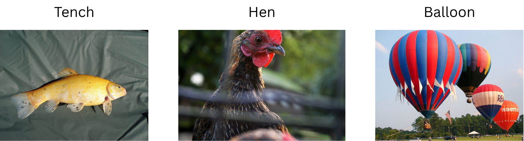
ImageNet is a database consisting of over 14 million natural images, each hand-labeled with a class corresponding to one of over 20,000 image categories, such as “baseball”, “birdhouse”, “strawberry”, etc. Here’s a sample of a few images from ImageNet:
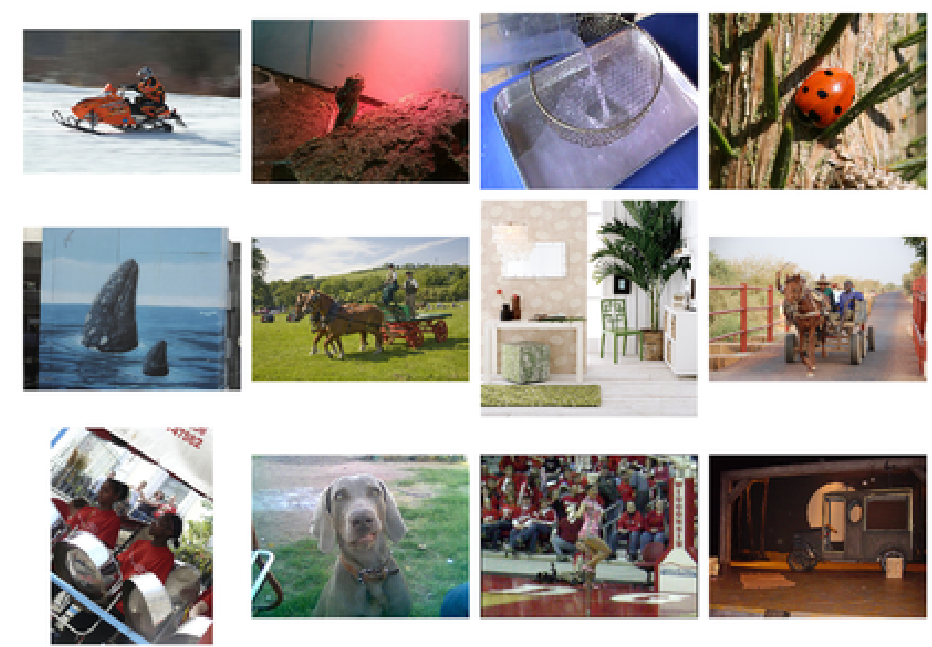
(Source: ImageNet Large Scale Visual Recognition Challenge. Original image author(s) unknown.)
In 2010, the ImageNet project began hosting an annual contest to see who could devise the best algorithms for various computer vision tasks derived from the ImageNet database, such as image classification (e.g., determine which images are baseballs, which are birdhouses, which are strawberries, and so on). This contest is called the ImageNet Large Scale Visual Recognition Challenge (ILSVRC).
In 2012, ILSVRC was won by a team of researchers at the University of Toronto including Alex Krizhevsky, Ilya Sutskever, and Geoffrey Hinton. Their submission, named AlexNet after Alex Krizhevsky, blew all the other submissions out of the water. It achieved a top-5 classification accuracy of 84.7%. In other words, given an image, the model predicted the top 5 image categories that it believed the image to belong to, and that top-5 list contained the correct category 84.7% of the time. This was over 10.8 percentage points above the top-5 classification accuracy of the second-place submission for the contest.
(Modern models can do better, but most of them build on the same ideas as AlexNet.)
AlexNet’s high performance can be attributed to a few things, but primarily: 1) it was a deep convolutional neural network (CNN); and 2) it made use of graphics processing units (GPUs) to make training feasible in a timely manner. Let’s focus on the former for now.
Convolutional neural networks employ a mathematical technique known as convolution (technically, they use cross-correlation, but we’ll treat these as the same thing). In essence, a CNN is like a multilayer perceptron, but its weights are organized into small blocks known as convolutional kernels (or, equivalently, convolutional filters).
For now, let’s assume that we’re working purely with grayscale (black-and-white) images. In such a case, you can imagine a convolutional kernel as a small grid, or “window”, of numbers, much like the representation of a grayscale image (but usually the numbers aren’t confined to a specific range, such as 0 to 1—they can even be negative). For example:
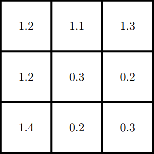
Although this is just a small 3x3 kernel, it can be used to “process” essentially every part of an entire grayscale image. This works by sliding the convolutional kernel across the image. For each patch of the image that the kernel slides over, a computation is performed: the inner product between the kernel and the image patch is computed, producing a single number as a result. Formally, an inner product is the sum of all element-wise scalar products between two tensors. Less formally, an inner product can sort of be thought of as a “similarity score” between the kernel and the image patch. If the image patch is “similar” to the kernel in some sense, then the number will be large and positive; if the kernel and image patch are very different from one another, then the number will be close to zero; and if the image patch’s values are completely “opposite” to those in the kernel, then the number may be large and negative. (That’s not exactly how it works, but this understanding is good enough for our purposes.)
A very nice visual demonstration of convolution by deeplizard can be found here. If you open the page and scroll down to the bottom, you’ll see an image of a handwritten 0 digit from MNIST labeled as the “input”. Each pixel is enlarged and its value, rescaled to be between 0 and 1, is displayed inside it.
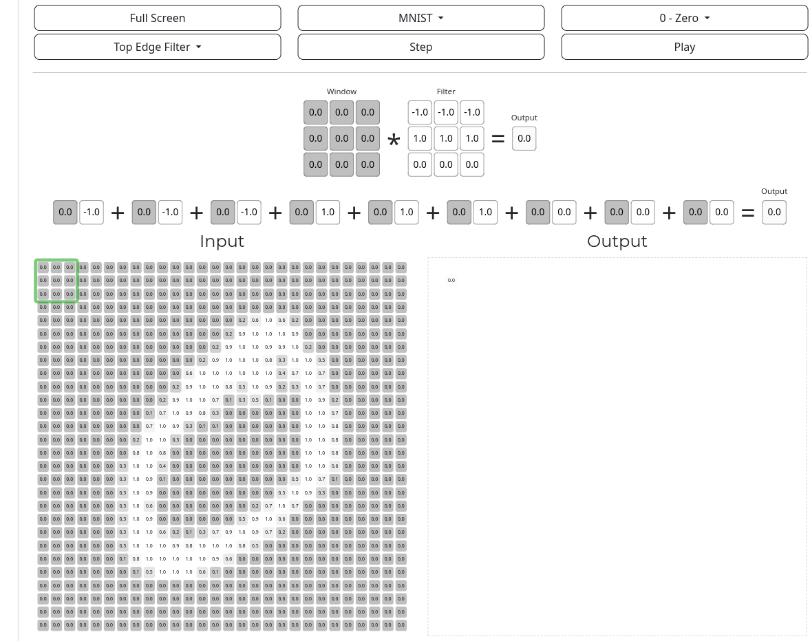
Above the input are the “window” and “filter”. The “filter” is the convolutional kernel, and the “window” is the patch of the image that the kernel is currently processing. When the “step” button above the diagram is clicked, the inner product (“similarity score”) between the kernel and image patch is computed and displayed in the corresponding part of the “output” diagram, and the kernel slides over to the next patch.
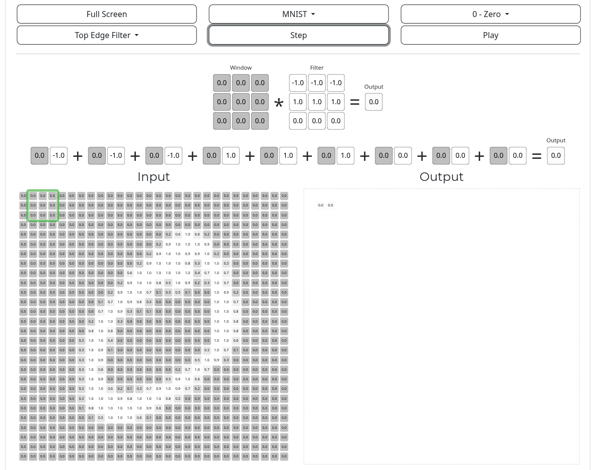
In the simplest case, the kernel slides over every patch in the entire image, and for each patch, it produces a single number as a result of the inner product computation. Since this happens for each patch in the image, this produces many numbers, and these numbers are themselves arranged into a grid. This grid of values is referred to as a feature map, and it can be visualized as a sort of image of its own.
In the above web demo, if you click the “play” button (next to the “step” button), it causes the convolutional kernel to step several times very quickly, sliding across and processing every patch of the input image. When its done, the output should depict a complete feature map:
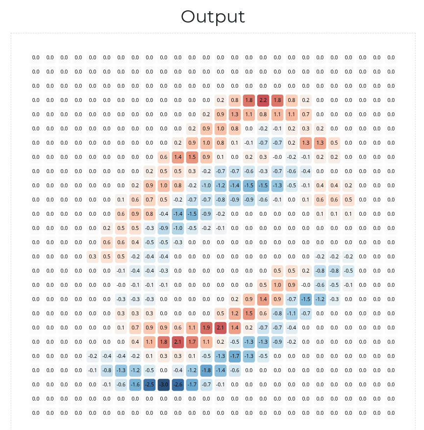
The large negative values of the feature map are colored in blue. The large positive values are colored in red. The values closer to zero are colored white. There’s a very important pattern here. Notice: the red-colored / positive values in the feature map correspond to the top edges of the handwritten 0 digit (i.e., edges that run along the top of the handwritten pen stroke), and the blue-colored / negative values correspond to the bottom edges:
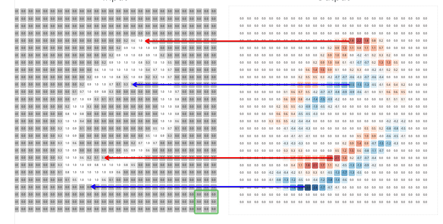
Indeed, the above diagram highlights the main idea of convolution: a given convolutional kernel is designed to look for a certain “visual pattern”. It scans over a given input image, and whenever it detects that pattern, it highlights it by producing a large positive value in the corresponding part of the output feature map. Whenever it detects the “opposite” of that pattern, it highlights it by producing a large negative value in the corresponding part of the feature map. For patches that are essentially unrelated to the visual pattern, it produces values closer to zero in the corresponding parts of the feature map.
This particular convolutional kernel is specifically designed to look for patches that have a row of black pixels immediately above a row of white pixels, hence why it highlights the top edges of the handwritten 0 digit via positive values in the feature map, and it highlights the bottom edges via negative values.
(In fact, if you know how inner products are computed, then you can even tell that this is what the convolutional kernel will do just by looking at its values.)
Depending on the exact values in the convolutional kernel, it may look for / highlight different kinds of visual patterns in the image. This one can detect horizontal edges, but a slightly different convolutional kernel might be able to detect vertical edges. Another might be able to detect topleft corners; another could detect topright corners; and so on.
This is how convolutional kernels work for grayscale images, but it turns out that the same idea can be applied to colored images as well. An RGB (colored) image is exactly like a grayscale image, except each pixel is represented by three values instead of just one. Hence, they can be processed by a convolutional kernel that, for each cell in the grid, also has three values instead of one. Such a convolutional kernel is often depicted as a 3-dimensional block of values instead of a 2-dimensional grid of values (the depth of this block corresponds to the number of color channels—3 in the case of RGB), but it slides over the image in the same way, processing each patch one at a time and producing a feature map as an output.
Convolutional neural networks (CNNs) are a kind of neural network, like an MLP, but they’re built primarily from convolutional kernels (and some other minor components that we won’t discuss). Research on CNNs actually dates back to the 1980s. The original CNN, coined the neocognitron, was published by Japanese AI researcher Kunihiko Fukushima in 1980. In 1989, Yann LeCun published LeNet-5, a CNN that was trained in much the same way as a typical multilayer perceptron. AlexNet further developed on these ideas.
So, how does a CNN work?
First, many convolutional kernels are created and combined into a so-called convolutional layer. By having many kernels, a single convolutional layer is capable of looking for many different visual patterns in a given image—not just one. For example, one kernel in the layer might look for vertical edges; another kernel might look for horizontal edges; another might look for topleft corners; and so on.
Each kernel in a convolutional layer scans over the given image and produces its own feature map. These feature maps are then stacked on top of one another into a 3D block (much like the input RGB image itself).
Here’s where things get complicated: a CNN typically does not have just a single convolutional layer, but rather many convolutional layers, and they’re arranged together in a sequence. Basically, the feature maps produced as an output of one convolutional layer are fed into the next convolutional layer as inputs. Perhaps this makes sense; feature maps can be visualized like images, so they can also be processed like images. Hence, a convolutional layer can analyze a feature map that was produced by another convolutional layer.
Below is a diagram of LeNet-5. It’s a smaller example, but notice that it has two convolutional layers (ignore the pooling and dense layers; they’re beyond the scope of this exploration).
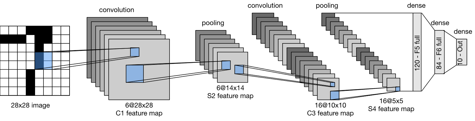
(Source: Wikimedia Commons. LeNet-5 architecture.svg. Authors: Zhang, Aston and Lipton, Zachary C. and Li, Mu and Smola, Alexander J. License: CC BY-SA.)
The first convolutional layer has 6 kernels (a “depth” of 6), hence why the first block of convolutional feature maps has 6 feature maps. The second convolutional layer has 16 kernels.
You might be wondering: why do CNNs use several convolutional layers arranged in a sequence? Well, think of it like this: the first convolutional layer in a CNN looks for simple, primitive patterns in the raw image, such as edges and corners. It then highlights those patterns in the corresponding parts of the various feature maps of its output. The next convolutional layer then looks for patterns within those patterns; it might look to see how edges combine together to form larger, more complex shapes, for example. The next convolutional layer further looks for patterns within those patterns, and so on.
The consequence is that very deep convolutional layers are capable of picking up on very abstract, high-level patterns present in the image—not just edges and corners, but entire objects like dogs and cats. When these deep layers discover these complex visual patterns, they produce large values in the corresponding parts of the various feature maps of their outputs. These values can then finally be used for various computer vision tasks, such as detecting the presence and locations of certain objects in an image (e.g., this image patch over here contains a dog; that patch over there contain a car; etc), classifying / labeling an image, and so on.
Here’s a very nice web demo by Adam Harley that lets you draw your own handwritten digit, and it displays various feature maps produced at various layers of a CNN trained to perform digit classification.
Because convolution works by sliding kernels across an image and applying them the same way to every patch, CNNs are naturally translationally invariant. That’s to say, unlike MLPs, their predictions do not vary drastically when an object is translated (shifted) slightly within an image (e.g., if your dog takes a step to the left, the CNN will still recognize it as a dog). After all, whether a given object is on the left side of the image or the right, the convolutional kernels will slide over it and detect it one way or another. This property, among others, makes them much better suited for computer vision tasks than a traditional multilayer perceptron.
So, CNNs are built from many convolutional layers, each of which contains many convolutional kernels, each of which is a small grid of numbers. But how are those numbers decided? Well, those numbers simply make up the weights of the CNN, much like the weights of a multilayer perceptron. Hence, they can be trained in the same way. That is, the convolutional kernels of a CNN are learned as a result of the training process.
Since these convolutional kernels scan over images to look for certain visual patterns, the CNN essentially learns what patterns to look for so as to accomplish its task (e.g., maximimizing classification accuracy / minimizing loss on the training set). For example, if the goal is to correctly classify dog vs cat images, then the CNN’s convolutional kernels might learn to recognize certain visual patterns that are common in images of dogs but not cats, and / or vice-versa, since the presence or absence of those patterns might provide a strong indication as to which class a given image belongs to.
The only issue is that tackling complex computer vision tasks often requires very big CNNs (e.g., CNNs with many layers, and / or CNNs with many kernels in each layer). Such large CNNs have many weights, so they’re slow to train and use.
Yann LeCun’s LeNet-5 was relatively small since it was just designed for handwritten digit and letter classification. AlexNet, on the other hand, needed to be able to distinguish, say, a German Shepherd from a Belgian Malinois (both are image categories in ILSVRC), which requires detecting much more complex visual patterns (many people would struggle at this task). Such complex visual patterns can be detected by CNNs, but it requires deeper convolutional layers. Hence, AlexNet was much larger than LeNet, making it much slower to train and use.
Alex Krizhevsky’s team addressed this problem by using Graphics Processing Units (GPUs) instead of Central Processing Units (CPUs) to train AlexNet. GPUs are a different kind of computer chip from a standard CPU. They’re designed a bit differently and are better suited for certain tasks, including training deep learning models on large data sets. This drastically sped up the training process. They weren’t the first to train deep CNNs with GPUs, but it was still a big deal because it proved that it was a viable strategy for solving complex, real-world computer vision tasks. Nowadays, it’s standard practice to train large deep learning models by using several GPUs in parallel.
CNNs have since been adapted for various other computer vision tasks beyond classification, and they’re ubiquitous in modern computer vision. For example, if you ask ChatGPT to caption an image for you, there’s a good chance that, under the hood, a convolutional neural network is being used to analyze the image. Convolution has even been adapted for generative computer vision tasks (e.g., generating images and videos).