Local Computation: Penalty Function Methods

---

Penalty function methods approximate a constrained problem by an unconstrained problem structured such that minimization favors satisfaction of the constraints.

The general technique is to add to the objective function a term that produces a high cost for violation of constraints. There are two types of methods:

• Interior penalty methods, also known as barrier methods
• Exterior penalty methods

General Form

minimize f(x)

subject to h(x)=0

g(x) <= 0

 We will reformulate f(x) such that the constraints are part of the objective function. We also want to insure that the two essential conditions of Lagrange's method hold:

1. If an optimal solution exists that requires the constraint to be tight, then any perturbation away from constraint activity should be heavily penalized.
2. If an optimal solution dictates the constraint be loose at optimality, the problem should behave as though it were unconstrained by that constraint.

The reformulated objective function:

minimize:

where:

f(x) is the original objective function

s= +- 1

t_i= scale factor for equality constraints

r_k= monotonically increasing or decreasing inequality scale factor

penalty function involving each original inequality constraint

penalty function involving each original equality constraint

 

This is a generalized equation that represents both interior and exterior methods. The nature of s, r and in the general formulation depends on whether one wishes to begin with a feasible solution and iterate toward optimality, or start with an infeasible solution and proceed toward both optimality and feasibility.

The equality scale factor, t_i, is the penalty for violation of an equality constraint. In the infinite barrier method, t_i would be set to infinity, approximated numerically by some large number such as 10²⁰. This method does not work well with inequality constraints.

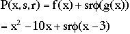
min f(x)= x² - 10x

subject to g(x)= x-3 <=0

Penalty method:

The nature of s and r:

If we set s=0, then the modified objective function is the same as the original.

If the constraint is "loose" (inactive) then (x-3) < 0

If the constraint is violated, then (x-3) > 0 and sr should be a large positive quantity in order to incur penalties.

If (x-3) = 0, then the value of s doesn't affect the solution. If s is positive unity (+1), given any particular value for r, the modified objective function is increased or penalized by any value of (x-3) not equal to zero.

The factor r can be interpreted as a scale factor that controls the actual effect of constraint violations. All cases can be dealt with by setting s= +1 or -1.

Both conditions are satisfied by the following formulation (referred to as the augmented objective function)

min P(x,r,s)= x² - 10x + sr(x-3)²

corresponds to

f(x) + sr(g(x))²

the penalty function is

this is known as the parabolic penalty method.

s is set to +1 because this is an exterior penalty method and the starting point is assumed to be infeasible.

If r=1, then the augmented objective function reduces to

min P(x,r,s)= P(x)= x² - 10x + (x-3)²

The optimal solution:

This solution violates the constraint. Our penalty scale factor r was not high enough. What if we set r= 100?

min P(x,r,s)= P(x)= x² - 10x + 100(x-3)²

with the solution:

As r -> infinity, x* -> 3, the true optimal solution. This suggests the exterior penalty algorithm. Start with r= e (the error) at the first iteration. If the constraint(s) is not violated, then you have the optimal solution. If the constraint is violated, increase the value of r until the optimal solution satisfies that constraint in terms of your acceptance criteria. The iterative solutions are always outside the boundary of feasible points. At each iteration the objective is increased but drawn closer and closer to the lowest feasible point.

1) Inverse penalty:

with s= +1

minimize:

2) Log penalty

with s= -1

minimize:

As r approaches zero, the solution vector approaches x*, the optimal constrained solution.

Consider the previous example, using the logarithmic penalty function.

The optimal value of x*= 3 can be approached by iteratively decreasing the value of r:

The augmented Lagrange multiplier method can be used for problems with equality constraints. Add a penalty term to the Lagrangian:

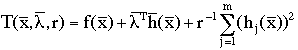
For this reduces to the exterior penalty method.

If we can find the exact solution to the minimization problem with finite r.

The augmented Lagrange multiplier method is iterative:

1) Assume and r.

2) Minimize and find .

3) Update and r.

4) Repeat until convergence

Summary

1) Penalty methods transform a constrained minimization problem into a series of unconstrained problems.

2) Exterior penalty methods start at optimal but infeasible points and iterate to feasibility as r -> inf.

3) Interior penalty methods start at feasible but sub-optimal points and iterate to optimality as r -> 0.

4) The methods are iterative, hence the term SUMT, Sequential Unconstrained Minimization Techniques.

5) We start with r reasonable because it makes the problem better conditioned (less sensitive to numerical round off, etc.) and hence easier to solve.

6) Exterior methods are generally more robust.