Running the Diabetes Experiment

In the Pima Indians Diabetes experiment, the goal is to compare three approaches to fitting a model:

• The Naive Bayes model
• A model found by a "hill climbing" search of the space of Bayesian networks
• A knowledge-based model

We would like to evaluate these models on small and large data sets to see if they give different results.

Obtaining and Preparing the Data

Download the diabetes.arff data file and save it in the weka-3-4/data folder.

These models require that the data be discretized. For our experiment, we will discretize each input variable into 3 ranges ("low", "medium", "high") by using an automated algorithm. This algorithm does not analyze the class variable (i.e., whether the person has or does not have diabetes). Here is the procedure:

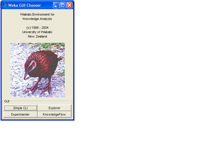
• Start WEKA. You will see the weka startup window:
  
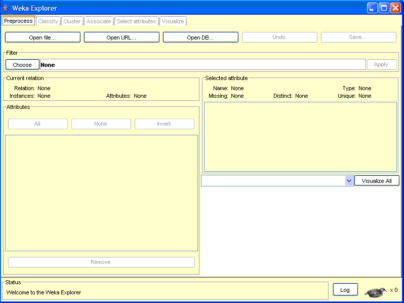
  Click on the Explorer button. This will bring up the main screen:
  
  

• Load the diabetes data by clicking on "Open file...", navigating to the data folder, and selecting diabetes.arff. The main screen should now look like this:
  

• Click on "Choose" in the "Filter" section. This will pop up the following menu:
  
  Click on the "+" beside "filters". Then click on the "+" beside "unsupervised". Then click on the "+" beside "attributes", and finally, click on "Discretize". The main screen should now show Discretize -B 10 -M -1.0 -R first-last in the area next to the "Choose" button.

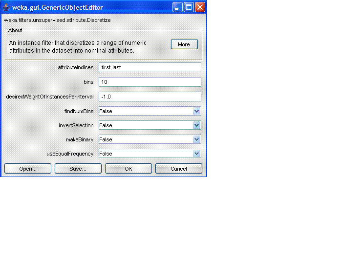
• Click on the "Discretize" text in this box. The following window should pop up:
  
  Set bins to be "3" and set "useEqualFrequency" to be "true". Then click "OK".

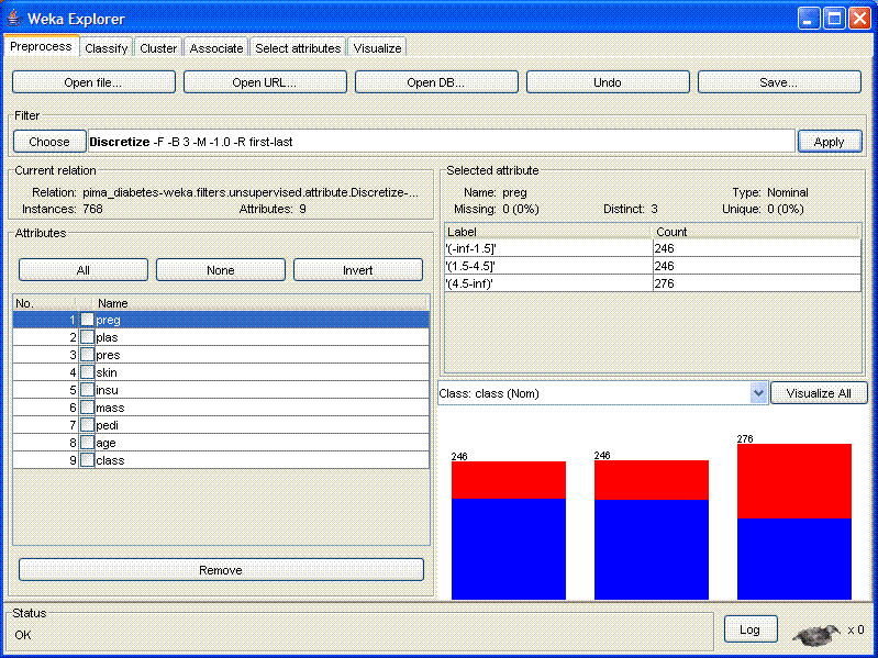
• Click the "Apply" button on the right-hand side of the main window. Your window should now look like this:
  
  The attributes have now been discretized.

Fitting Bayesian Networks to the Data

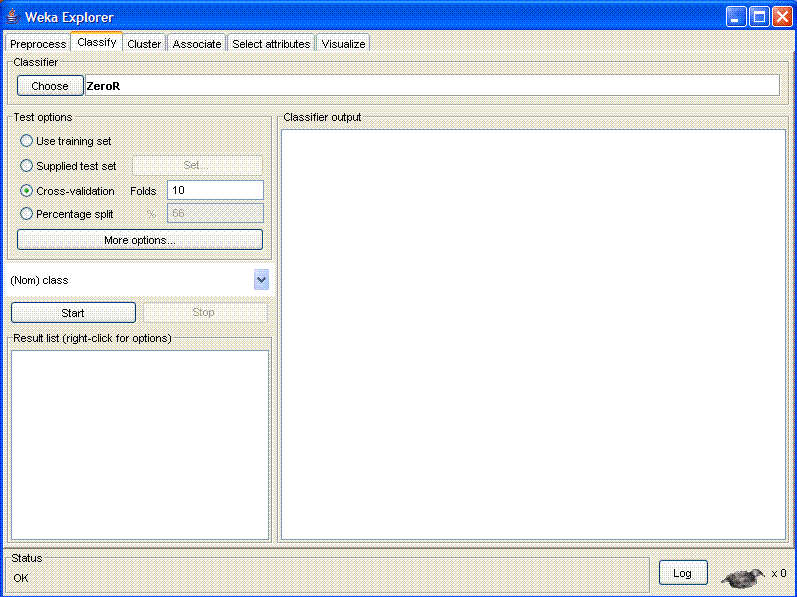
• Now click on the "Classify" tab at the top of the window. This will change to the classification page. It should look like this:
  
  

• Now click on the "Choose" button in the "Classifier" section. In the menu that pops up, click on the "+" next to "Bayes" and then click on "BayesNet". Now the area to the right of the "Choose" button should contain a long string of text that begins BayesNet -S -D -B -Q.

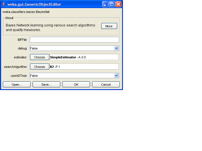
• Click on this area to bring up the properties menu for the BayesNet classifier:
  
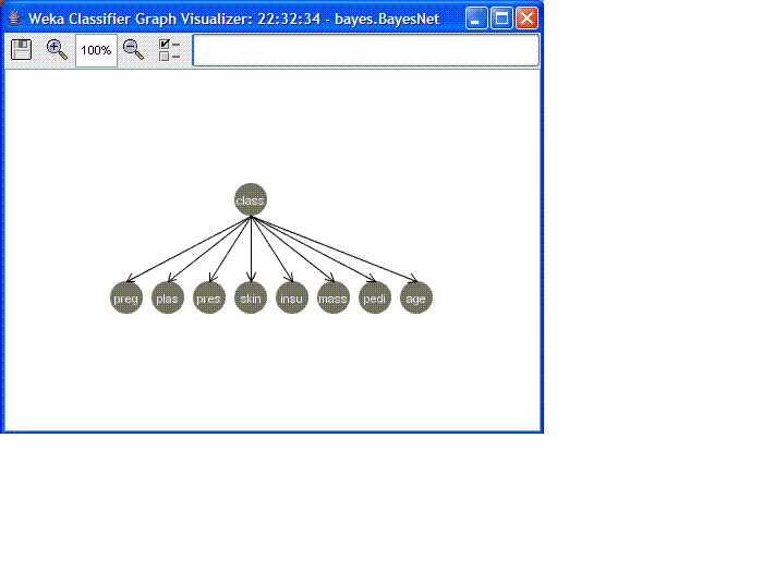
  What we do at this point depends on which of the three model-fitting methods we are going to use. Let's start with the Naive Bayes approach. In this approach, the Bayesian network consists of one edge from the class node to each of the other variables.

  To choose this structure, click on the "Choose" button next to "searchAlgorithm". Click on the "+" next to "Fixed" and choose "Naive Bayes". Then Click "OK" on the properties menu.

• Now turn your attention to the "Test options" section of the window. This gives us various options for how to evaluate the quality of the model after it is fit to the training data. We will use the "Percentage split" option, so click on the button next to it. The "%" box should now be "un-grayed-out". By default, it says we will use 66% of the data for training and therefore 34% for evaluation. To test how well Naive Bayes will work on small samples, we will test two values for this number: 10% and 80%. So for now, erase the "66" and type "10" into this box.

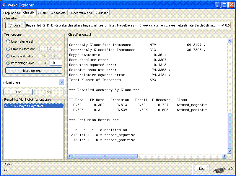
• We are ready to run the algorithm. Click the "Start" button. Two things will happen. First, a line will appear in the "Result list (right-click for options)" area. Second, there will be a lot of text in the "Classifier output" window. Here is what my window looked like at this point:
  
  Note that there were 213 incorrect-classified instances, which gives an error rate of 30.7803%. At the bottom of the window is the "Confusion Matrix":

     a   b   <-- classified as
   314 141 |   a = tested_negative
    72 165 |   b = tested_positive
  

  The rows in this matrix correspond to the correct classes (a = does not have diabetes; b = has diabetes). Hence, there are a total of 314 + 141 = 455 patients without diabetes in the test data, and 72 + 165 = 237 patients with diabetes. The columns correspond to the predicted classes. Hence, 314 of the 455 negative patients were correctly classified as negative and 141 of them were incorrectly classified as positives (called "false positives"). This gives a false positive rate of 0.31. Conversely, 72 of the 237 positive patients were falsely classified as negatives (called "false negatives") and 165 were correctly classified as positives.

• We can visualize the Bayesian network by right-clicking on the highlighted line in the "Result list" window and then selected "Visualize Graph". The resulting graph looks like this:
  
  

• Now close this window and go back to the "Percentage split" box and set it to 80. Click "Start" again. You should see that the error rate is now substantially lower. Also note that we now have only 105 negative cases and 49 positive cases in our test data set. Record the error rate for later plotting.

• Now let's evaluate how well a "knowledge-based" Bayesian network will work. To do this, download the file diabetes.xml and save it in a convenient folder. This file describes the structure of the network.

  Now click on the BayesNet -S -D -B stuff to the right of the "Choose" button in the BayesNet classifier to bring up the properties of the BayesNet classifier. Again click on the "Choose" button for the "searchAlgorithm". This time, select "FromFile". This will fill in the text "FromFile -B" in the box next to the "Choose" button. Click on this text, and you should see the following properties box:
  
  In the "BIFFile" box, type the path name for the "diabetes.xml" file. For example, mine was "C:/diabetes.xml". Now click "OK" to close this properties menu and "OK" to close the BayesNet properties menu. Set the Percentage Split back to 10, and click the "Start" button. Record the results. Then set the percentage split to 80, click the "Start" button, and record the results.

• Now let's evaluate how well a hill-climbing search works. Again, click on the "BayesNet -S -D -B" stuff next to the "Choose" button in the "Classifier" section. The properties window for BayesNet will pop up. Again, click on the "Choose" button for "searchAlgorithm". This time, click on the "+" next to "local" and select "HillClimber". 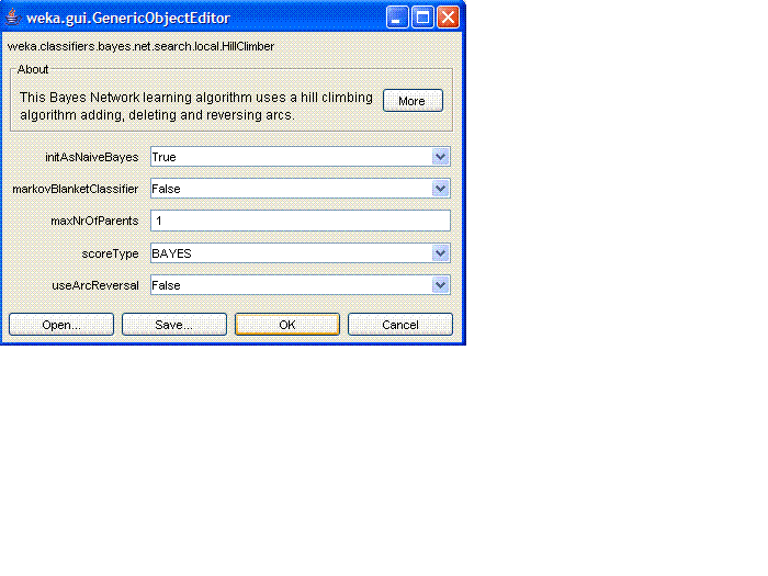This will fill in the text "HillClimber -P 1 -S BAYES" for the "searchAlgorithm". Click on this text to bring up the properties box for the HillClimber, which looks like this:
  
  Set "initAsNaiveBayes" (i.e., initialize the network to have a Naive Bayes structure) to "False", set "maxNrOfParents" (maximum number of incoming arrows to a node) to 3, and set "useArcReversal" (consider reversing arcs during the search) to "True". Then click "OK" to close this menu, and "OK" again to close the BayesNet menu.

• We are ready to run the HillClimber algorithm. Set the "Percentage Split" to 10, click "Start", and record the results. Then set the "Percentage Split" to 80, click "Start" and record the results.

In my experiments, I found that the HillClimber worked best for both large and small samples, that Naive Bayes was second best, and that the knowledge-based network structure was the worst. You may want to repeat the experiments with different percentage splits to see whether this result holds up across the whole range. I suggest that you record your data in a spreadsheet and plot learning curves for each of the three methods.