|
|
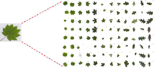
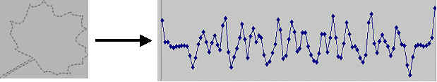
Figure 1: Image processing for isolated leaf |
There are two modules in the implementation. These modules run in batch mode. The first one performs basal image processing. It extracts features that describe the shape of the leaves. The second module embeds the dynamic program and performs the stint of template matching and species prediction.
The following configurations have been
considered:
Training and testing the system with only isolated leaves
Training with isolated leaves and predicting species of herbarium samples
Training with herbarium samples and predicting species of isolated leaves
The features extracted by the first module are the angles measured at each pixel point along the boundary of the leaves. The actual procedure for extracting these angles is described later. The angles recorded along a boundary form a sequence, which is input to the dynamic program. The output of the dynamic program is the cost of the best path match between two streams corresponding to the two leaf-shapes being compared. To predict the species of an unknown leaf, the leaf shape is compared to all template leaves using the dynamic programming algorithm. The K best matches are selected. Each of the K nearest neighbors votes in favor of its (annotated) species, and the species that gets the most votes is predicted to be the species of the input (unknown) leaf shape.
Color
segmentation is performed to separate out the leaf pixels from the background
pixels. The scanned pictures of the leaves are not void of dust, seeds, and
other particles. Filtering is required to remove this unwanted noise. A
morphological operator called erosion was applied to remove pixels
corresponding to such noise. The images are converted to a matrix of binary
values 0 and 1 or ON and OFF. ON corresponds to pixels
belonging to the leaf area, and the rest of the cells in the matrix are OFF
(see figure 1). For each island of ON pixels, its boundary is extracted.
|
|
Figure 1: Image processing for isolated leaf |
|
|
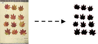
Figure 2: Image processing for herbarium
samples
|
The
procedure for navigating the boundary starts by scanning from pixel (0,0) –
left to right, bottom to top – until it finds the first leaf-pixel, i.e. a
pixel that is ON. It extracts all boundaries in the anti-clockwise
direction. To do this, at each pixel it keeps track of the direction followed to
reach that pixel. The direction at the start pixel is RIGHT (At each
pixel, one of four directions is possible – RIGHT, LEFT, UP and DOWN).
Depending on the current direction, a search is done for the next boundary pixel
in the counter-clockwise direction. The trace ends when we return to the start
pixel. Each closed boundary that is extracted from the image is called an
island.
The
island boundaries that are significantly smaller compared to the size of the
whole image are rejected. Specifically, a boundary of size less than one-tenth
the height of the entire images may be considered insignificant.
|
Search
in raster order for first pixel that is ON Case
RIGHT: if
(P[i+1][j-1]=ON) {direction=DOWN; P[i+1][j-1] is the next pixel} Case
LEFT:
if (P[i-1][j+1]=ON) {direction=UP; P[i-1][j+1] is the next pixel
} Case
UP:
if (P[i+1][j+1]=ON) {direction=RIGHT; P[i+1][j+1] is the next
pixel } Case
DOWN: if
(P[i-1][j-1]=ON) {direction=LEFT; P[i-1][j-1] is the next pixel } |
Boundary
extraction algorithm
|
The pseudo code above outputs the coordinates of the pixels along the boundary of the leaves. The coordinates are converted into a stream of angles before applying the dynamic programming algorithm. Figure 3 shows how this conversion is done. At each pixel, we construct a polygon approximation of the local curvature and measure the exterior angle A as shown in figure 3. To obtain the exterior angle at pixel i along the boundary, we compute the angle between the line segment joining pixel i to pixel i-10 and the line segment joining pixel i to pixel i+10. The sequence of angles measured along the boundary in counter clockwise direction gives a one-dimensional stream representation of the boundary.
 |
Figure
3: Angle measurements along the boundary
|
|
|
|
Figure 4: Scalar representation of boundary |
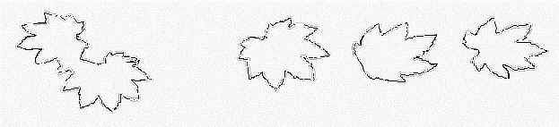
Pattern matching for leaf-shape recognition should obey following two rules:
It
should be invariant to translation, rotation and scaling of the shapes.
It
should be able to handle deformities, occlusions and overlaps.
The first rule is
required of any shape matching technique. The second condition is a special rule
necessary for the digital images obtained from the herbarium. No two leaves of
same species have exactly similar shapes. Some leaves might be deformed, folded
or even overlapping. These distortions have to be handled.
The Dynamic Time Warping (DTW) algorithm is a good general approach for matching similar signals. It can be used to compare objects with stored templates. Only, a good one-dimensional representation for two-dimensional shapes is required. Scalar transformation of Cartesian representation of the boundary into a one-dimensional signal generally filters out the location information. Rotation of the original shape results in a cyclic shift in the one-dimensional representation.
Ideas
from DNA (biological) sequence matching algorithm can be borrowed to allow
multiple gaps and occlusions. A dynamic programming algorithm for matching
whole, partial and overlapped shapes is shown below. The term Qi,k
determines gaps in one of the sequences. For each gap, a penalty wk
proportional to the length of the gap is added to minimum distance path. The
term Si,j, which is split into terms Pi,j
and Ri,j, allows overlaps, i.e. allows the same part of the
second pattern to match multiple parts of the first pattern.
| Algorithm Let A=a1a2…aM
and B=b1b2…bN be the two sequences to
be compared Qi, j = Min [ Di,k
+ wk ]
and wk = W4k
(u≥0, v≥0) is the linear gap penalty for a gap of
length k Si,j can be split into two
terms Pi,j and Ri,j Thus, |
Dynamic
Program for shape recognition
|
This algorithm just like the earlier algorithms iterates MN times. In each iteration, minimum of five terms, viz. Di-1, j-1 , Di-1,j + W1 , Di,j-1 + W2 , Si,j , Qi,j , must be calculated. By an inductive process, Si, j (i.e. Pi, j and Ri, j) , Qi,j can be calculated in single step as shown below. Thus, each iteration executes in constant time, and the algorithm runs in O(MN).
|
Qi,j
= Min [ Di-1,j + w1 ,
Min ( Di-k,j + wk ) ] Si,j
= Min [ Pi, j , Ri,j ] Pi,
j = Min [ Dk,j-1 ]
+ W3 Similarly, |
|
Inductive calculation of Si,j and Qi,j |
Figure below illustrates the significance of such an algorithm. It shows matching of an isolated whole leaf template with two unknown overlapping leaves. Note the unknown pattern is along the horizontal and the known pattern is along the vertical. Initially, the minimum distance path consists of cells corresponding to matching elements of the isolated leaf pattern with the left side leaf of the two overlapped leaves. The first three terms in calculation of Di,j determine this path. Then there is a jump (made possible by terms Pi,j and Ri,j) in the path, and the isolated leaf pattern starts matching the boundary of right side leaf. The figure also illustrates the wrap around. Finally, the overlapped area of the two leaves does not match anything on the isolated leaf and hence results in a gap. The gaps can be attributed to term Qi,j in calculation of Di,j. The minimum distance path starts from the first column and terminates at the last column. The cost of the minimum distance path is the minimum of all Di,N values in the last column.
W1 and W2 should be set to small values. A small value larger than zero makes diagonal moves preferable. Constant W3 determines the threshold for gap inclusion. W4 assures that there are no arbitrary jumps in an attempt to match the same part of known sequence with different parts of the unknown sequence.
The dynamic programming
algorithm described above compares the stream of angles obtained for given input
leaf against all of the templates in the library i.e. the training set. The cost
of the minimum distance path for each match is calculated. Finally, the K
best matches, i.e. the templates that give minimum cost are picked out. A
majority of the retrieved images is expected to belong to the same species as
the unknown leaf. The retrieved images vote in favor of their (annotated)
species, and the species that gets the most votes is predicted to be the species
of the unknown leaf shape.