\(\DeclareMathOperator*{\argmax}{\mathrm{argmax}}\) \(\newcommand{\best}{{\mathit{best}}}\) \(\newcommand{\back}{{\mathit{back}}}\)
Knapsack: Unbounded, 0-1, and Bound
Knapsack is a group of classical problems that can be solved by DP.
There are three versions of knapsack:
Which version is the easiest? Which version is the hardest? Before thinking algorithmically, just think about real-life experience of going shopping.
Well, intuitively, shopping at Costco must be a lot easier than shopping at a local convenience store, because in the former you only need to care about your bag (your only constraint) and not the store (if you like something, you can take as much as you want), whereas in the latter you also need to keep track of the state of the store (“are there still apples left?”), or in other words, you have both the bag capacity constraint and the product availability constraint. Naturally, with more constraints, optimization is harder. Indeed, we will see below that unbounded is much easier to solve algorithmically than 0-1 or bounded.
Between 0-1 and bounded, which one is even harder? Well they are about the same level, because you can convert one to the other and vice versa. If you can solve bounded, then you can obviously solve 0-1 which is a special case; but if you can solve 0-1, you can also use it to solve bounded by converting a bounded problem to a 0-1 one: You can duplicate items in a bounded store, e.g., a “three-apple and two-orange” store can be converted to a 0-1 store with 5 items, [apple1, apple2, apple3, orange1, orange2].
Therefore, unbounded is the easiest, and 0-1 and bounded are about the same level (with the latter just a tiny bit more involved).
This store has \(n\) products, each with a weight \(w_i\) and value \(v_i\), and each has infinite number of copies. How can you maximaze the total value of products that can fit your shopping bag of capacity \(W\)? You can also view weight \(W\) as your budget and each weight \(w_i\) as the price (which is certainly different from its value to you, \(v_i\); e.g., some products are “overpriced” and of little value or interest to me). For example, \(W=6\), and there are 3 products:
| \(i\) | name | \(w_i\) | \(v_i\) | \(v_i/w_i\) |
|---|---|---|---|---|
| 1 | apple | 2 | 3.2 | 1.6 |
| 2 | orange | 5 | 9.0 | 1.8 |
| 3 | pear | 4 | 7.0 | 1.75 |
Note that the weights must be integers but values are real numbers.
If we are greedy, we would always pick the product with the highest value (orange) or the highest “value per weight” (still orange), but then our bag can’t fit any other product. So you got a total value of 9.0.
Instead, we can fit three apples in our bag, which gives a total value of 9.6; or even better, we can fit one apple and one pear, which gives a total value of 10.2. So clearly greedy is not optimal.
How would you solve this problem using DP?
Again, think divide-n-conquer: if you can’t solve the problem for a big bag of capacity \(W\), can you solve a similar but smaller subproblem?
So let’s define \(\best[w]\) to be the best value for a bag of capacitiy \(w\ (0\leq w \leq W)\). For such a bag \(w\), we can try to put every single product \((w_i, v_i)\) into it and thus shrinking it to an even smaller size \(w-w_i\) but with the reward of \(v_i\), so:
\[ \best[w] = \max_{i=1\sim n, w\geq w_i} \best[w-w_i] + v_i\]
base case: \(\best[0] = 0\); actually not only that, but if a bag is too small for any item, then it must be value 0 as well:
\[ \best[w] = 0\quad (0\leq w < \min_i w_i)\]
This simple algorithm has space complexity \(O(W)\) (number of subproblems or table entries) and time complexity \(O(W n)\) (for each subproblem, there is a loop over each \(i\)).
Let’s look at the above example for \(W=6\). If you do bottom-up, you would fill
each \(\best[w]\) for \(w=1,2,3,4,5,6\) (in that order); but you do
top-down, you would start with \(w=6\)
by calling best(6), and try \(i=1\) first, which calls
best(4), which in turn calls best(2), etc.
Here is the full recursion tree:
              best(6) = 10.2      -           -
        i=1 /           /   |i=2  |     \i=3   \
           /      +v_1 /    |     |+v_2  \      \+v_3
      best(4)= 6.4 -> 7     best(1)=0     best(2)=3.2
  i=1 /   /     \i=3   \
     /   /+v_1   \      \+v_3
best(2)=3.2       best(0)=0
i=1|    |
   |    |+v_1
best(0)=0
You notice that best(3) and best(5) are
never asked (not to mention solved). Why? Because they are not
needed for the global problem best(6), and top-down only
asks questions on-demand. If top-down asks best(i), then
that subproblem must be potentially useful for the global
problem. In this sense you can also view top-down as “lazy”; you’ll find
that in computer science, being lazy is one of the highest virtues, and
all clever algorithms are lazy.
This example suggests that top-down often solves less subproblems than bottom-up which is “blind” about the future when solving each subproblem one-by-one. To make it more extreme, let’s \(\times 100\) for each \(w_i\) as well as \(W\):
| \(i\) | \(w_i\) | \(v_i\) | \(v_i/w_i\) |
|---|---|---|---|
| 1 | 200 | 3.2 | 1.6 |
| 2 | 500 | 9.0 | 1.8 |
| 3 | 400 | 7.0 | 1.75 |
Now bottom-up still needs to solve all 600 subproblems (\(w=1,2,3,4,...,600\)) without knowing the vast majority is not useful. How many would top-down solve? Still just 4 (this time we draw the recursion tree horizontally):
  +------------v
  |            v
600 -> 400 -> 200 -> 0
  |                  ^
  +--> 100 --------->^
So which order is faster? It depends on the input. If the input is very sparse so that very few subproblems are solved, then top-down is a lot faster; if the input is very dense so that most subproblems are solved, then bottom-up is slightly faster (due to avoiding the overhead for recursion).
As always, each DP problem has a graph interpretation. For MIS, it’s the longest path between source (base case) and target (global subproblem); for Fibonacci or number of bitstrings, it’s the number of paths between source and target.
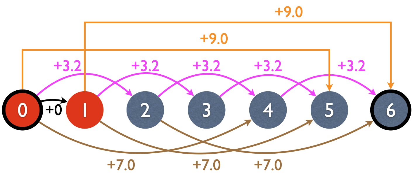
For unbounded knapsack, like MIS, it’s also the longest path between source and target, the only difference being the graph structure. In MIS, each node (subproblem) has two incoming edges (in graph terminology, we say each node has an in-degree of 2), which correspond to the two choices per node (take or not take \(a_i\)). For unbounded knapsack, however, each node \(\best(w)\) has (at most) \(n\) incoming edges, which correspond to each possible product. Here is the DP graph for the running example:
Based on the graph structure, we can figure out the backpointer. In MIS, since each node involves a binary decision, the backpointer for each node is also a boolean. But for our problem, since each node faces a multiple-choice decision, the backpointer will need to remember which item to take (i.e., the best \(i\), or the best incoming edge among all \(n\) of them. Note that in the mathematical notation, the backpointer is always just replacing the \(\max\) in \(\best(...)\) with \(\argmax\).
\[ \back[w] = \argmax_{i=1\sim n, w\geq w_i} \best[w-w_i] + v_i\]
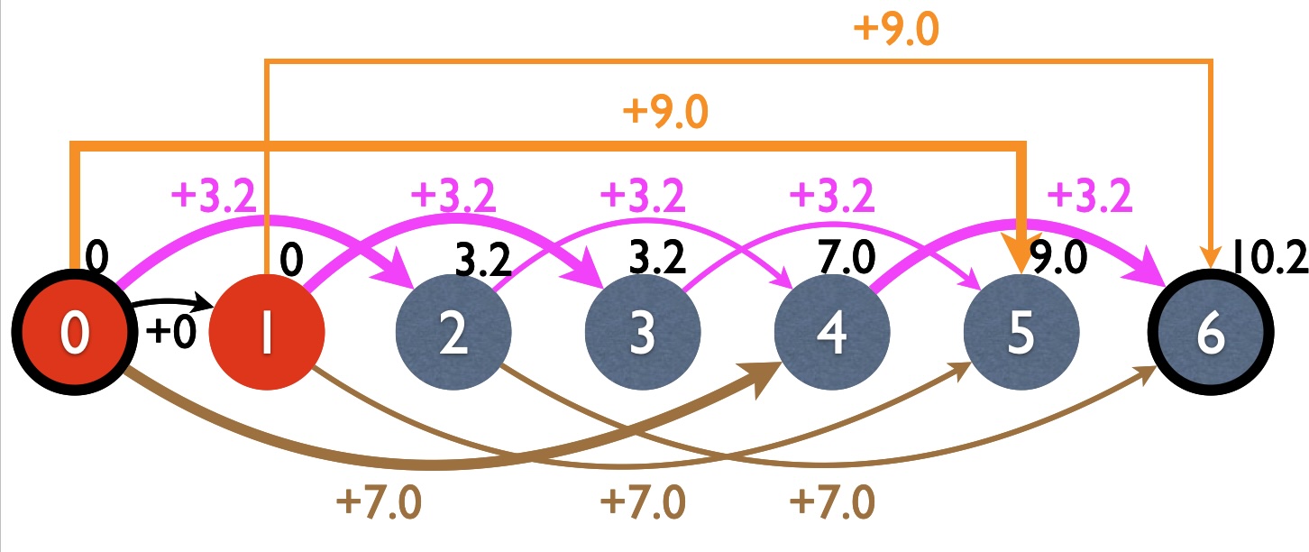
Here is the DP graph after bottom-up, with backpointers in bold edges. Note that each subproblem (i.e., node) is solved, with the best value written in black just above the node.
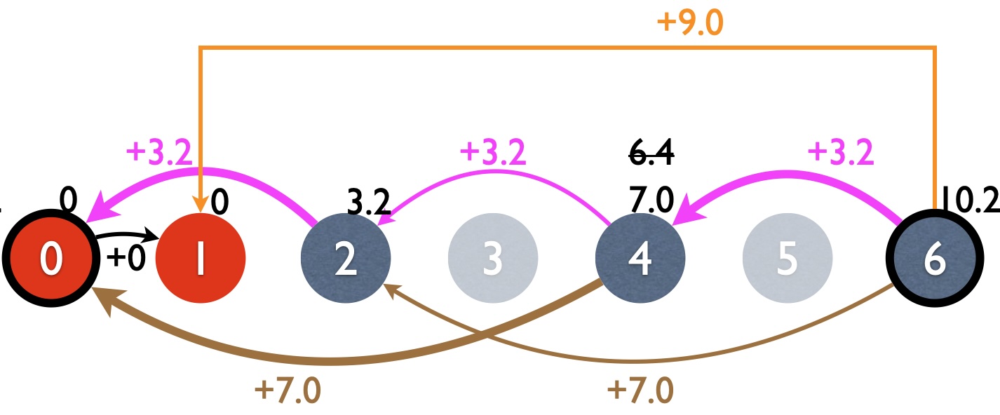
Finally, here is the DP graph after top-down recursion. Note that some nodes (3 and 5) are never visited because they’re not needed by the global problem. Here I reversed the edge directions to reflect the recursive calls (see recursion trees above). Backpointers are indicated by bold edges.
In DP, the space complexity is always the number of subproblems (or size of the table for memoization, or number of nodes in the DP graph). So for unbounded, it’s \(O(W)\). The time complexity is basically the space complexity times how many choices you have per subproblem, which is equal to the number of edges in the DP graph. For unbounded, each subproblem faces a multiple choice decision over (at most) \(n\) items and therefore each node has indegree at most \(n\) in the DP graph, so the time complexity is \(O(Wn)\).
Now you are back from Costco and enter a local convenience store where each item has only one copy. As discussed above, planning shopping in this setting is much harder than the unbounded case because now you also have the product availability constraint and therefore need to maintain the state of the store (as well as the state of the bag). Naturally, this means your subproblem should not be a one dimensional \(\best(w)\), but two dimensional
\[\best(w, ???)\]
wotj the “\(???\)” being the “store” dimension. The big question is, what information should we put in that dimension?
A first thought is that we should represent the state of the store by
a bit-vector (or boolean array), with each bit corresponding to one
product: 1 means that item is still available and 0 means it’s already
taken, e.g., 100 means “the apple is still there but the
orange and the pear are already taken”. Equivalent, you can have a set
\(S\) for the remaining items as the
second dimension.
This method is certainly correct, but then this second dimension would have \(2^n\) possibilities (2 choices per item, or the total number of subsets is \(|2^{\{1,...,n\}}|=2^n\)), which means that the new space complexity would be \(O(W \cdot 2^n)\). That’s way too slow due to the exponential growth: \(2^{10} = 1024\), and \(2^{20} \simeq 10^6\). Can we make it faster by avoiding \(2^n\)?
For the second dimension, think about the MIS problem in Sec. 2.1, which is also a subset optimization problem (with the additional constraint of “independent subset”). In total, there are also \(O(2^n)\) possibilities, but you can solve it in \(O(n)\) time by considering “take” or “not take” for each item \(i\) sequentially. Each time you shrink the problem by one (or two) item(s). In terms of subsets, instead of enumerating all \(2^n\) subsets, the MIS algorithm only considered the following \(O(n)\) ones:
         {} -- best[0]
        {1} -- best[1]
      {1,2} -- best[2]
        ...
{1,2,...,n} -- best[n]
Same idea here. You enter a 0-1 store and you say to the owner “your store is too big for me to solve and I’m going to divide-n-conquer (actually decrease-n-conquer) and I’ll shrink your store by one item”. Let’s say you take a bag of size \(w\) and enter a store of items \(\{1,2,\ldots, i\}\). You have two possible actions:
This binary decision on item \(i\) is very similar to the MIS case, with the only difference being in MIS if you take \(i\) you have to go to \(i-2\).
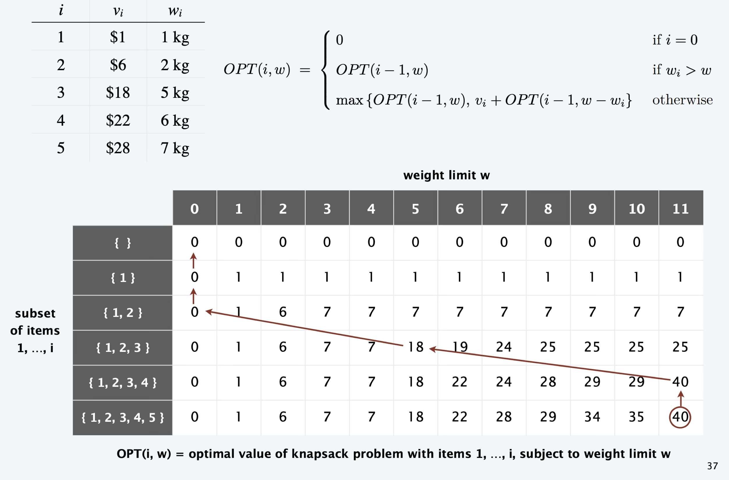
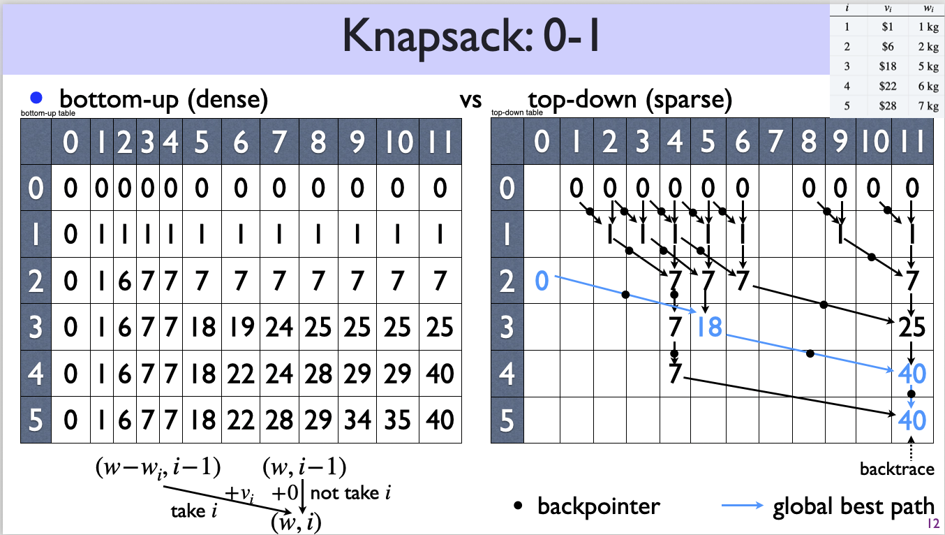
More formally, we define \(\best[w][i]\) as the best value for a bag of \(w\) in a store of items \(\{1,\ldots, i\}\), and it can be solved recursively:
\[ \best[w][i] = \max \begin{cases} \best[w-w_i][i-1] + v_i & w\geq w_i \\\best[w\qquad][i-1]\end{cases}\]
Base cases:
Space and time complexities:
Unlike all previous DP graphs that are one-dimensional, now we have a two-dimensional graph, since our subproblem has two dimensions. Each node in the 0-1 knapsack DP graph is \((w, i)\), which has two incoming edges (binary decision):
The goal is to find the longest path from any base case subproblem \((0, i)\) and \((w, 0)\) to the goal subproblem \((W, n)\).
Here top-down is generally much faster because most subproblems are not visited in top-down.
The most advanced and general version of knapsack is bounded, where each item \(i\) has \(c_i\) copies. It subsumes both unbounded (\(c_i=\infty\) for all \(i\)) and 0-1 knapsack (\(c_i=1\) for all \(i\)) as special cases.
The general idea is almost identical to 0-1 knapsack, i.e., we still define the subproblem as follows:
\(\best[w][i]\) is the best value for a bag of \(w\) in a store of items \(\{1,\ldots, i\}\) where each item \(i\) has \(c_i\) copies.
But instead of a binary decision (take or not take \(i\)), we now face a choice of how many
copies of item \(i\) we want to take,
as long as it is between 0 and \(c_i\)
and fits the bag, i.e., over the range of \([0, \min\{c_i, \, \lfloor w/w_i
\rfloor\}]\) (or in Python 3 notation,
range(min(ci, w//wi))).
\[ \best[w][i] = \max_{j=0\ldots \min\{c_i,\, w/\!/w_i\}} \best[w - j \cdot w_i][i-1] + j \cdot v_i\]
Notice that this formula is even simpler than the 0-1 case as \(j=0\) corresponds to the not-take case.
The space complexity is still \(O(Wn)\) since we did not change the subproblem definition.
The time is a bit tricky, where a naive analysis would end up \(O(W n \max_i c_i)\) because for each \((w,i)\) subproblem you have the innermost loop of \(j\) over (worst-case) \([0, c_i]\). But each \(c_i\) is different, so we use the max over all \(c_i\) as an upperbound (since big-O notation is about upperbound). But that’s too crude because using the max \(c_i\) for all \(i\) severely overcounts. To be more accurate, each \((w,i)\) subproblem (\(w=1\ldots W\)) has the \(j\) loop over \([0,c_i]\), so all those subproblems combined cost \(O(W c_i)\); taking the sum over different \(i\), we have \(O(W \sum_i c_i)\) (note there is no \(n\) here – it is implicit in the \(\sum\) loop). Alternatively, you can say the \(n \max_i c_i\) part should be replaced by \(c_1 + c_2 + \ldots c_n = \sum_i c_i\), so the correct time complexity is \(O(W \sum_i c_i)\).
The above time complexity would be more obvious if you consider the
following alternative solution of bounded knapsack: you convert a
bounded problem to 0-1 by duplicating each item \(i\) \(c_i\) times. For example, if there are 3
apples, make them apple_1, apple_2, and
apple_3, each with a unique copy. Now you have a 0-1 store.
How many items does this 0-1 store have? Well, \(n' = \sum_i c_i\). So the new 0-1
problem can be solved in \(O(Wn')=O(W
\sum_i c_i)\) time which is identical to our analysis above.
However, the drawback is that this alternative solution has a larger space complexity \(O(W \sum_i c_i)\) as opposed to \(O(Wn)\).
This is very similar to the 0-1 graph, except that each node \((w,i)\) can have up to \(c_i + 1\) incoming edges (the 1 being not-take). Still, top-down should be much faster than bottom-up for this problem in general.
Here is an ASCII diagram summarizing the three versions of knapsack:
unbounded (w) * MIS (i) = 0-1 (w, i)
0-1 (w, i) * #_of_copies = bounded ((w, i) = max_j)

          unbounded: best[w] = max_i best[w-w_i] + v_i
              multiple-choice: take which item?
             +--------------------------------+
    b     {} |                                |
 M  i    {1} |  0-1: best[w][i] = max {., .}  |
 I  n  {1,2} |  binary choice: take i or not? |
 S  a   ...  |                                |
(i) r {1..n} |                                |
    y        +--------------------------------+
                              |
                              v
   bounded: best[w][i] = max_j best[w-j*w_i][i-1] + j*v_i
      multiple-choice: take how many copies of i?