The first major achievement in symbolic AI ever since the official birth of AI in 1956 is General-Purpose Problem Solving formulated as AI search, and its applications in games such as Chess.
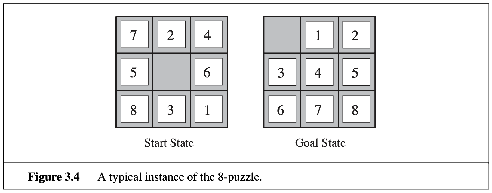
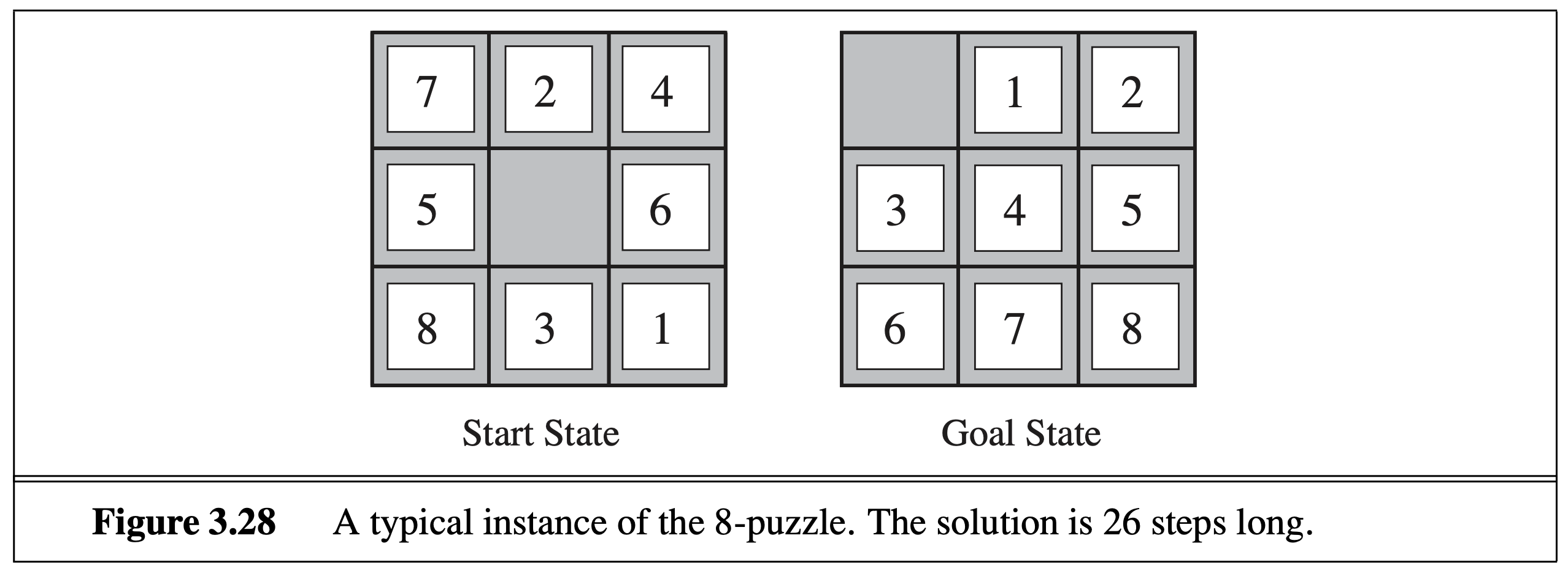
It turns out that many seemingly hard problems (esp. puzzles) can be formulated as a search problem, to find a path (or the optimal path under some path cost function) from a start state to a goal state that satisfies the goal condition. For example, in the famous 8-puzzle game, you’re given a (random) start state such as (7 2 4 5 _ 6 8 3 1), and your job is to find a series of operations that eventually lead to the goal state where the space is at the top left corner: (_ 1 2 3 4 5 6 7 8). The allowed operations (or “actions”) are just the swaps between the space and one of its neighboring numbers. For example, from the above start state, you can swap 2 with the space and produce: (7 _ 4 5 2 6 8 3 1). It seems ridiculously hard to find a solution, so AI search is here to help you! AI search will not only find a solution, but will also find the shortest solution (least number of steps).
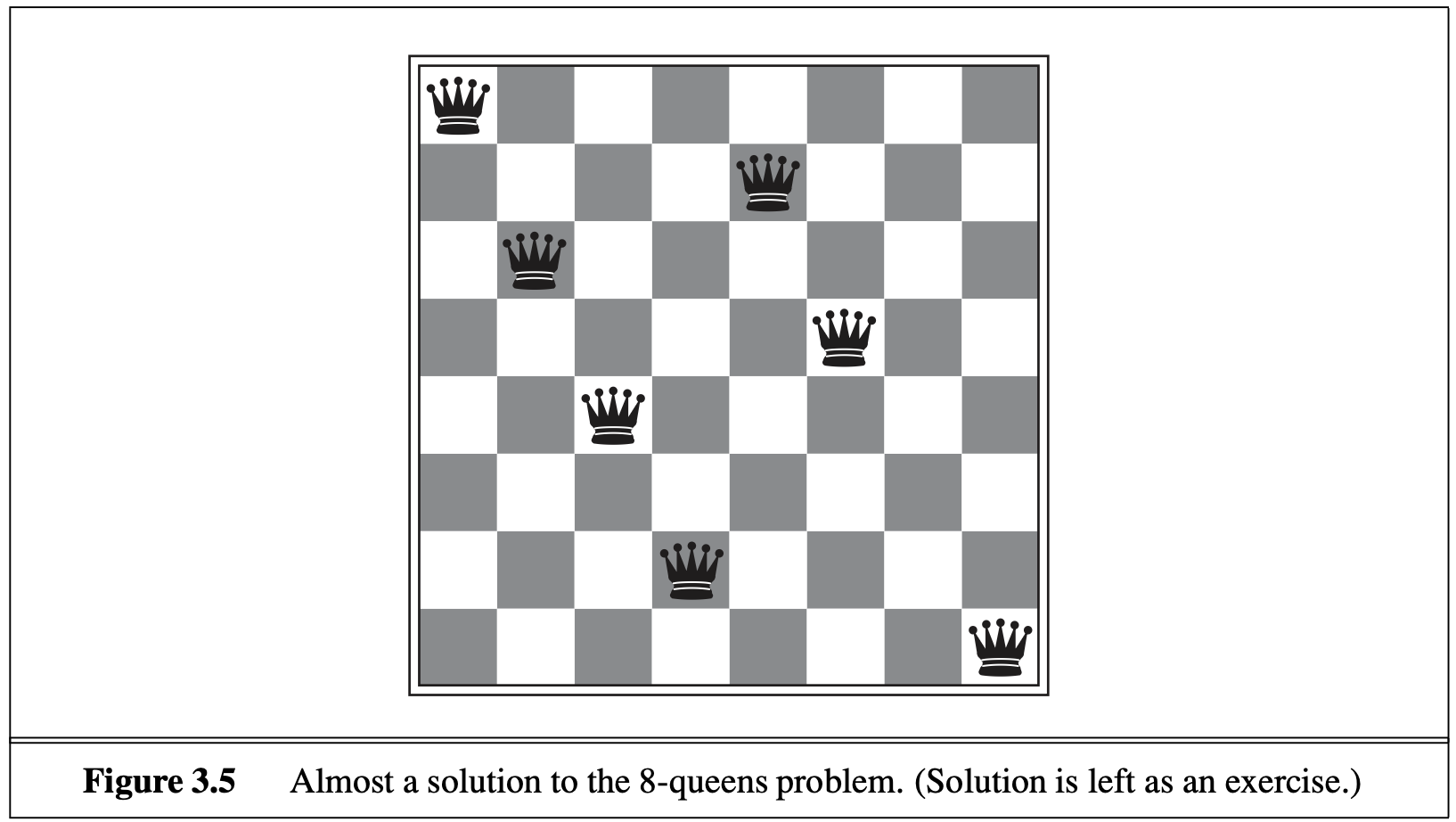
Another famous game is the 8-queens puzzle: how to place 8 queens on a chess board without any queen attacking another queen? Your job is to incrementally place one more queen on the board without it attacking any existing queen. Keep doing that and see if you can have 8 queens on board. It is very likely that you got stuck in the middle and need to backtrace.
In general, to formulate a problem as search you just need to formally define the following things (known as “abstraction” of the problem):
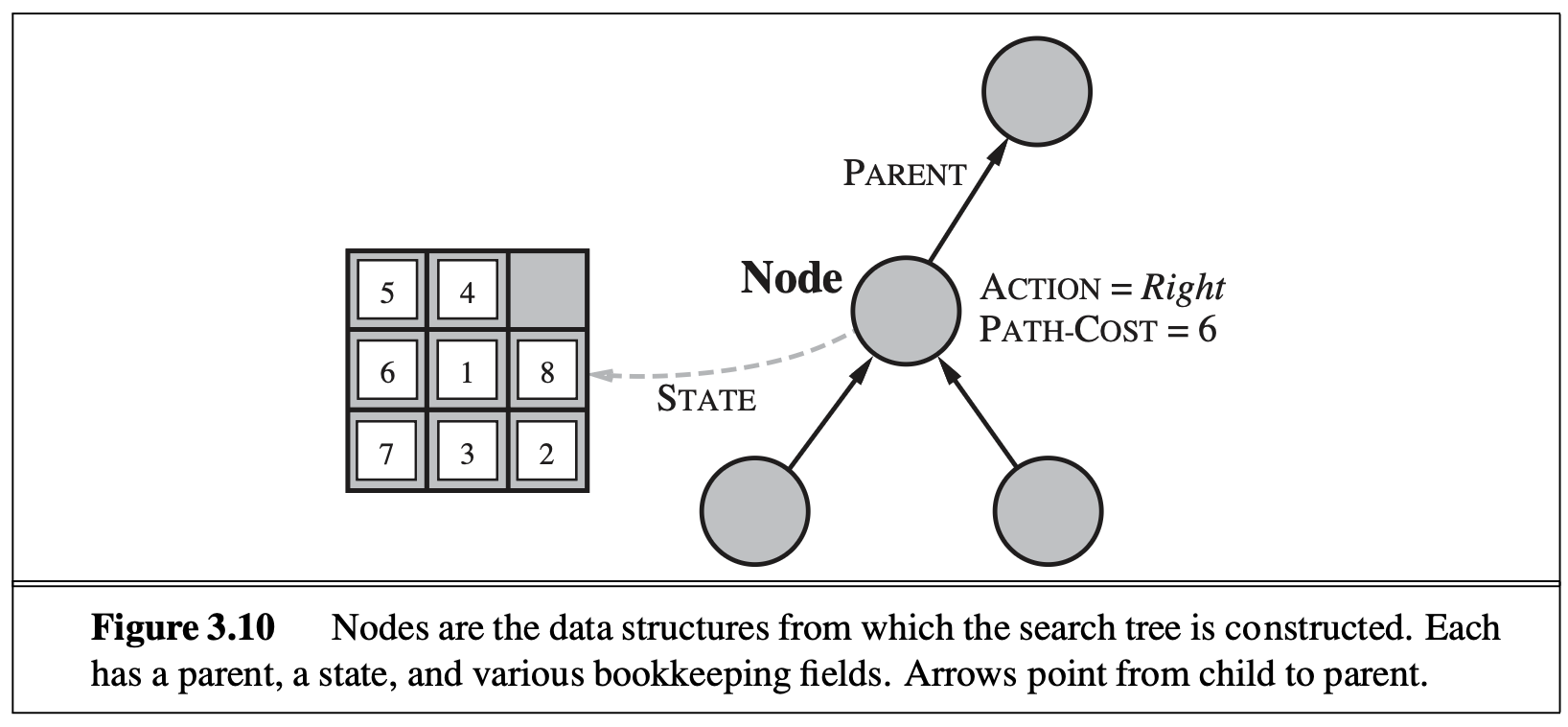
If we view this formulation from a graph perspective, then each state is a node (or vertex) in the graph, and each transition is an edge from the previous state to the next state. Your job is to find a path (or the shortest path, or all paths) from the start node to a goal node.
For many problems, the search graph degenerates into a search tree (tree is a special type of graph) if after branching, the two branches will never encounter the same node. For example, in the 8-queens, if we restrict our actions to be “placing a queen on the next row without attacking existing queens in previous rows” (i.e., adding queens row-by-row), then we guarantee that from each state, two actions will have completely different descendant nodes, so the search graph is a search tree. However, in 8-puzzle, we can never guarantee that, because two sequences of moves can lead to the same state.
The two widely used basic search algorithms are breadth-first search (BFS) and depth-first search (DFS). They both belong to the categoary “uninformed search” which contrasts with “informed” or “heuristic” search to be discussed below. In other words, BFS and DFS are kind of “blind search” or “brute-force search”.
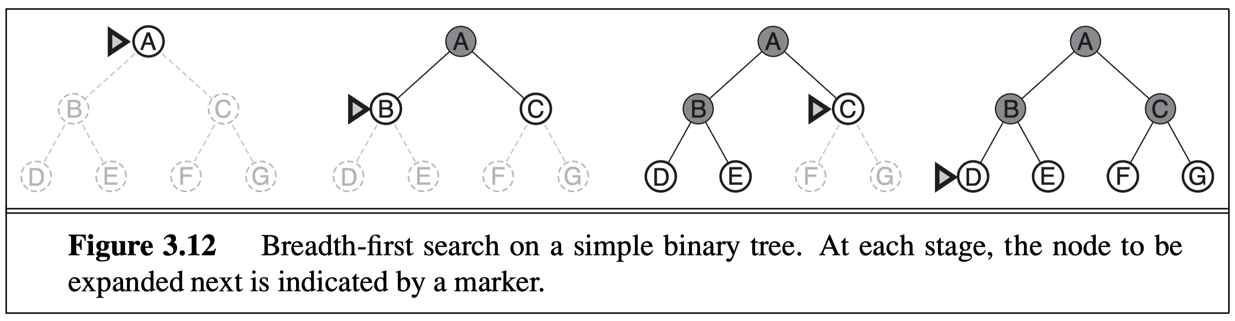
BFS simply explores the search graph or search tree in a “broad” way, and always expands the shallowest node in each step. It is implemented by a queue data structures which is first-come-first-serve (FCFS) or first-in-first-out (FIFO). Each time
The nice property of BFS is that for uniform-cost path (e.g., in 8-puzzle, each move is of cost 1), the first time BFS finds a goal state, it is guaranteed to be the optimal (shortest) path. This does not hold if each move has different cost, but we can modify BFS to best-first search (see below) to accommodate that (by replacing the queue with a priority queue).
The problem of BFS is the exponential explosion of storage requirement in memory. This is obvious: for a search graph with a branching factor of \(b\) (\(b=4\) in 8-puzzle and \(b=8\) in 8-queens), the first level has 1 node (start state), the second level has \(b\) nodes, the third level has \(b^2\) nodes, and the \(i\)th level would have \(b^i\) states. This expansion grows too fast and BFS quickly runs out of memory for most search problems.
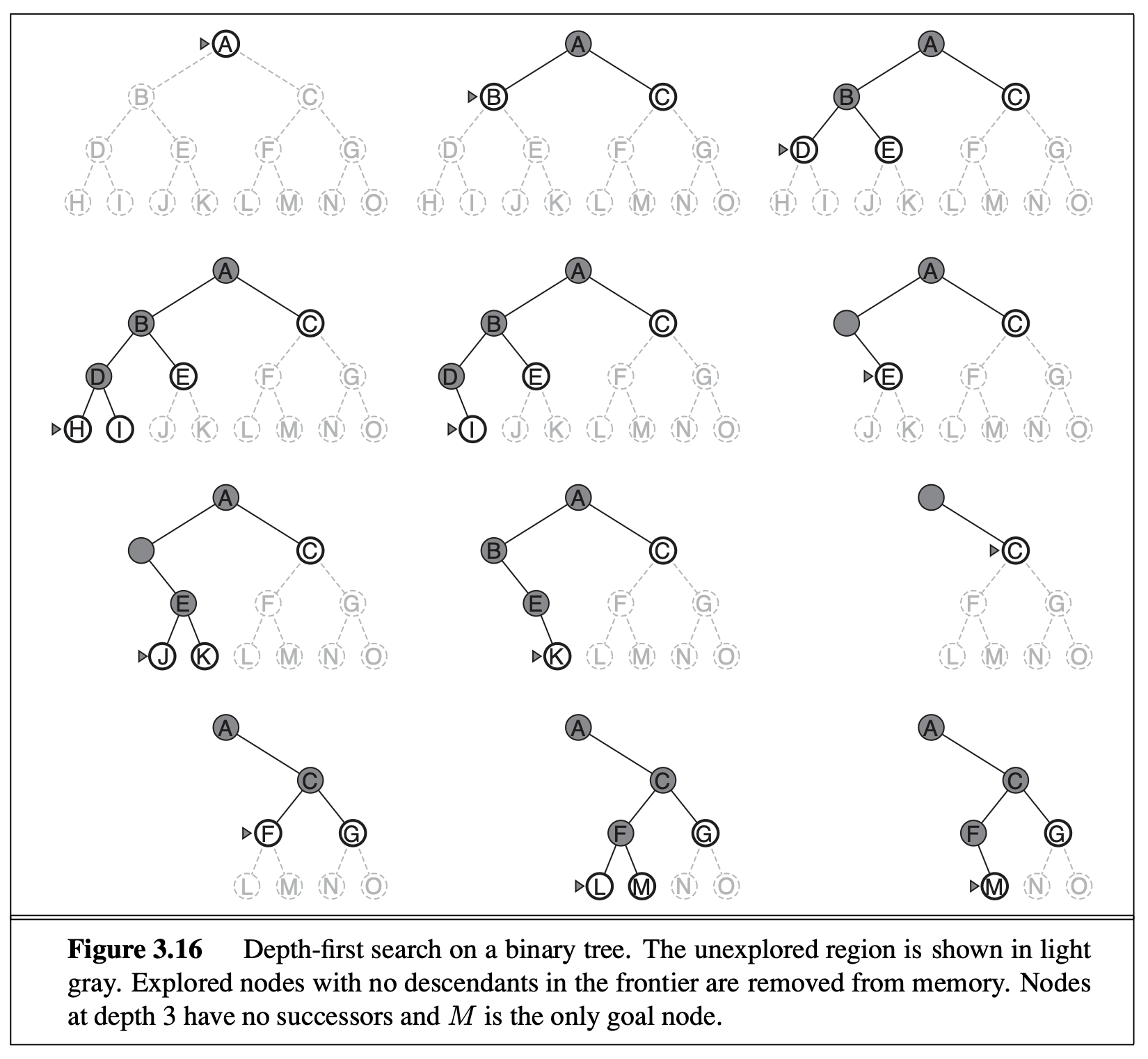
DFS, on the other hand, expands the deepest node in each step. It doesn’t have the exponential explosion problem that BFS has, because DFS only needs to store the active path. To implement DFS, we either use a stack (first-come-last-serve, FCLS, or first-in-last-out, FILO) or recursion (which is implemented by a stack under the hood). DFS is very similar to human search: from each state, we try a move and enter the next state, and keep going until we reach the goal state or got stuck in a dead-end, in which case we backtrack.
The problem of DFS is that it does not guarantee that the first goal state found has the optimal path, because other paths (to be explored later) might be shorter. For this reason, if you need optimal path, DFS has to explore all possible paths, which takes exponential time.
Vanilla BFS costs too much memory and vanilla DFS takes too much time. So AI researchers developed improved methods that address these limitations.
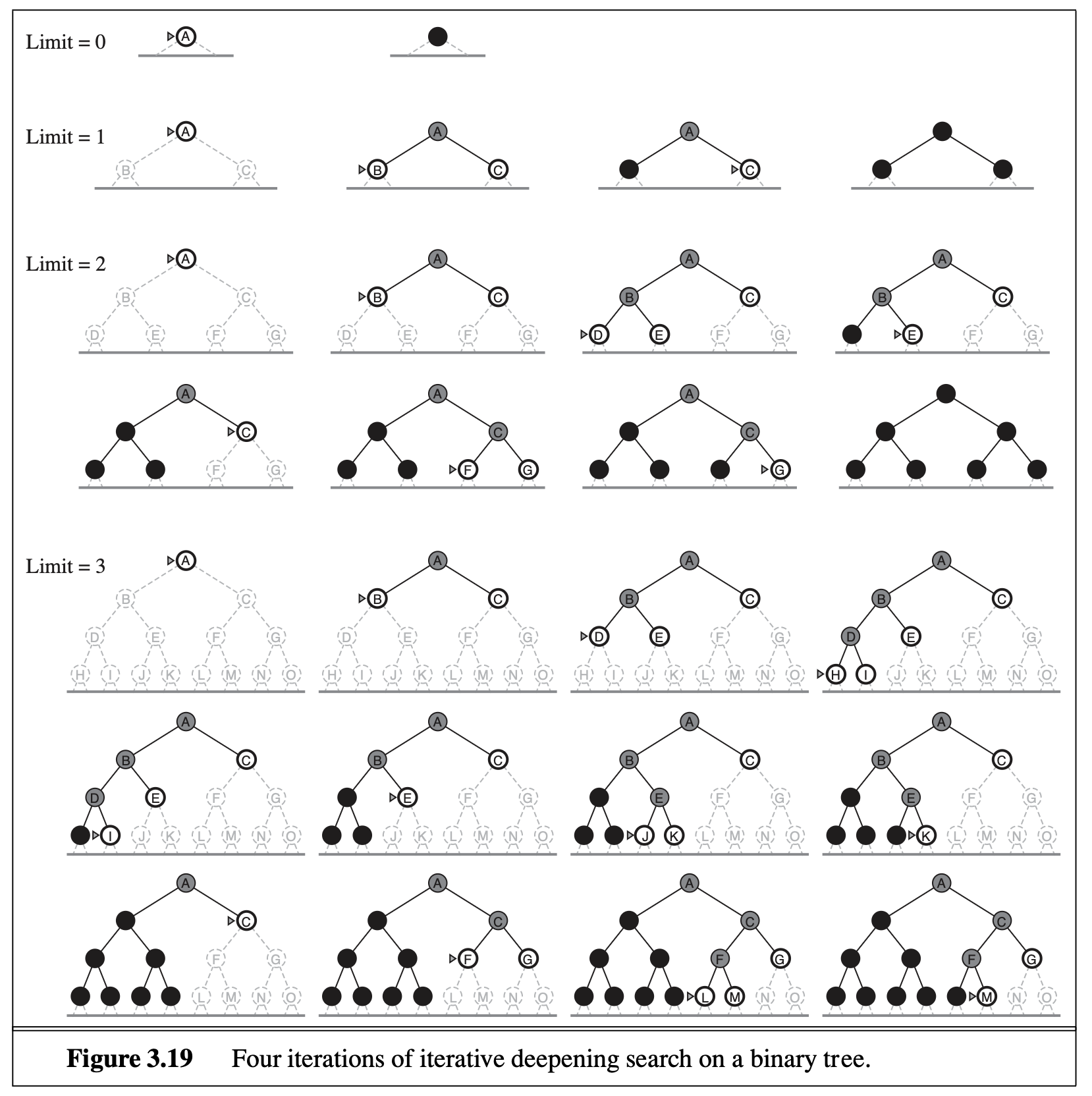
One possible way to improve DFS and avoid searching the whole graph for theoptimal path is “iterative deepening DFS”, which essentially combines BFS and DFS. The idea is simple: first allow DFS to search up to 1 level deep. If it doesn’t find a goal state, we allow DFS to search up to 2 levels deep. If it still doesn’t find a goal state, do DFS up to 3 levels deep, and so on. The good thing is that once you find a goal state, you can stop immediately and claim this is the optimal (shortest) path. The drawback is that some time is wasted in repeated searches. For example, level 2 search includes level 1 search; level \(i\) search includes level \(i-1\) search. However, this repetition is negligible given the exponential explosion, because each level is \(b\) times more nodes than the previous level (\(b\) is the branching factor). You can think of iterative deepening DFS as a hybrid that uses BFS globally (level progression) and DFS locally (within a level), and it combines the merits of both BFS and DFs.
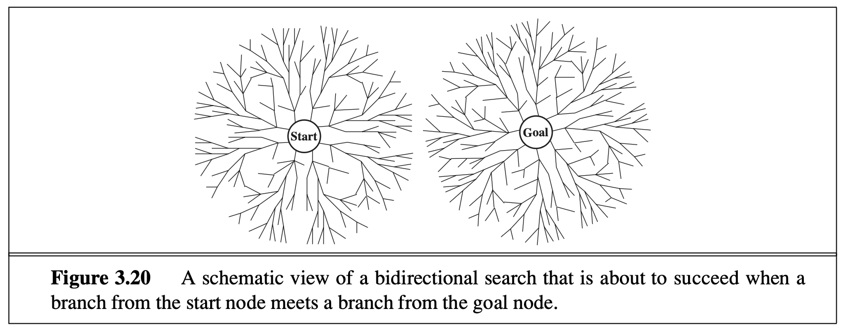
One possible way to improve BFS is bidirectional search, one forward search from the start state, and one backward search from a goal state (if only works for predefined goal states). If they meet somewhere in the middle, you can stop the search and claim optimal path. This method often significantly improves the search efficiency if there is “inverse” action for each action.
The above search algorithms are still mostly “blind search”, and not very intelligent. Next, AI scientists developed informed search (also known as heuristic search) that are more intelligent. This is usually considered the first non-trivial milestone in the history of symbolic AI.
The general approach here is best-first search, which has a cost for each node expanded, and will always expand the lowest cost node, because low-cost nodes are more likely to lead to optimal solutions. Best-first search is in spirit very similar to BFS, but in order to know which node has the lowest cost in the queue, we need to replace the strictly first-come-first-serve queue by a priority queue. A priority queue is like the queue in a hopsital emergency room (ER), which is not ordered by the time of arrival, but rather by urgency.
However, if you think of 8-puzzle, the cost of each node is just the number steps taken, then best-first is no different from BFS. How can we do better?
Well, besides the cost so far (from start state to here), we should also think about how many steps there will be to a goal state. Apparently, some states are much closer to the finish line than others. For example, in 8-puzzle, if a state has most numbers in the correct place and only a couple of misplaced numbers, then intuitively thinking, it is very promising and probably doesn’t need too many more steps to finish. By contrast, if a state has all the numbers out of place and very far from their target position, like a random permutation, then you need many more steps to finish.
So the idea is to estimate the remaining cost to goal. Of course you can’t estimate it very accurately, but the more accurate your estimate is, the faster the search. This is the idea of A search* (pronounced “A-star search”), the most famous AI search algorithm. It evaluates nodes by combining \(g(n)\), the cost from start to node \(n\), and \(h(n)\), the estimated cheapest cost to the goal:
\[ f(n) = g(n)+h(n) \]
This \(h(n)\) is known as the heuristic function. Now if we do best-first search based on \(f(n)\) instead of \(g(n)\), provided the \(h(n)\) satisifies certain simple condition, then the first solution A* search finds is guaranteed to be optimal (just like BFS and best-first).
What condition do we need for the heuristic function \(h(n)\)?
Very simple: as long as it does not overestimate the true cost to the goal, i.e., it can be “optimistic” and underestimate. For example, we can set \(h(n)=0\) for all \(n\), and then A* search degenerates into best-first search.
As an example, let’s reconsider the above idea of estimation for 8-puzzle. We can define two different heuristic functions:
\[h_2 =3+1+2+2+2+3+3+2=18.\]
Clearly, \(h_2\) is also optimistic, because all any move can do is move one tile one step closer to the goal (in reality you need many more moves).
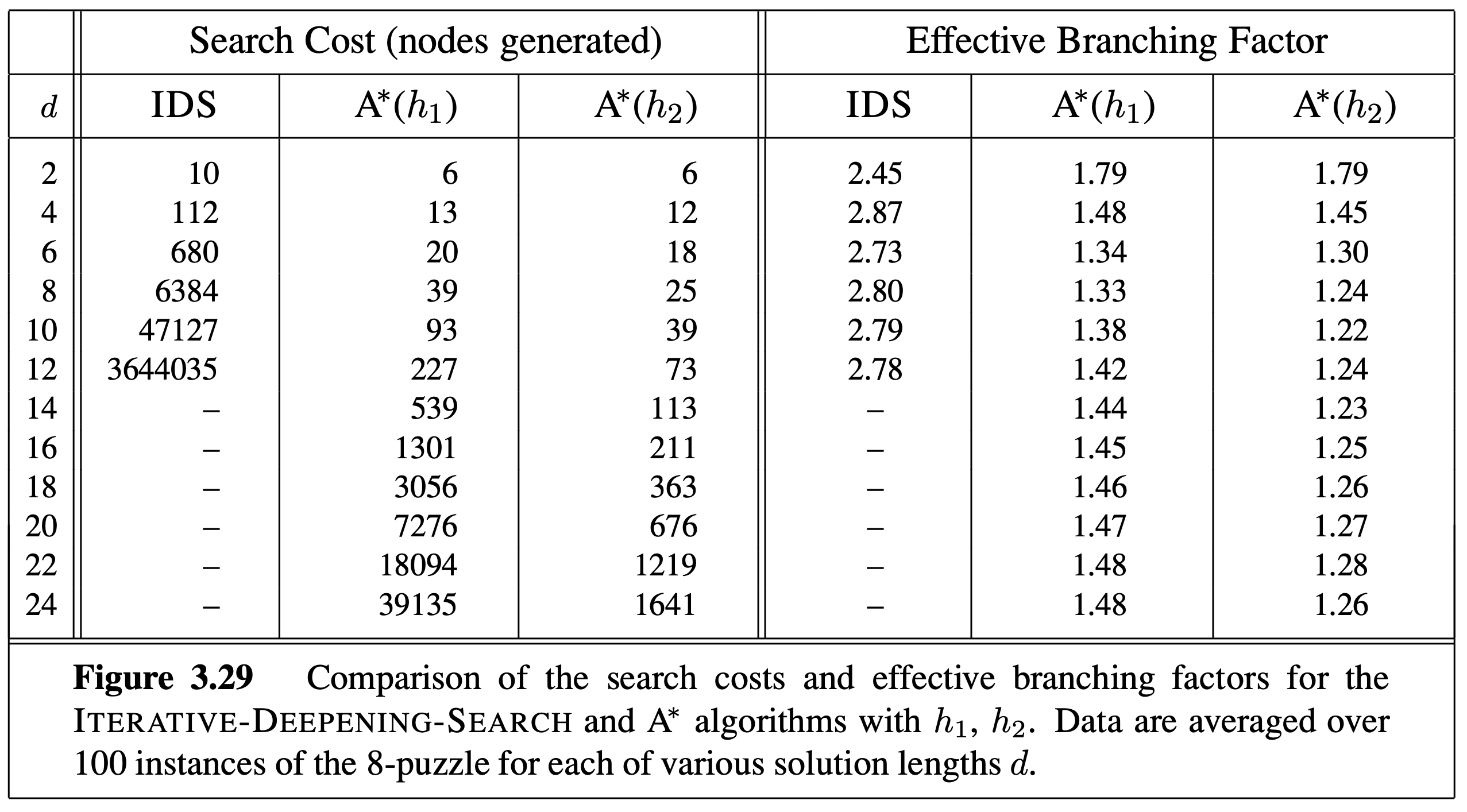
The actual best path has 26 steps, and as expected, neither \(h_1\) or \(h_2\) overestimates the true cost. \(h_2\) is a more accurate estimate (actually, for any state, \(h_2\geq h_1\)), and surprisingly, it only overestimates a little bit for our case. This suggests that using \(h_2\) can speed up the search much more substantially than using \(h_1\) (although the latter already brings significant speed up), as shown in the table below.
The art of A* is to come up with more and more accurate but optimistic heuristic functions to speed up the search.
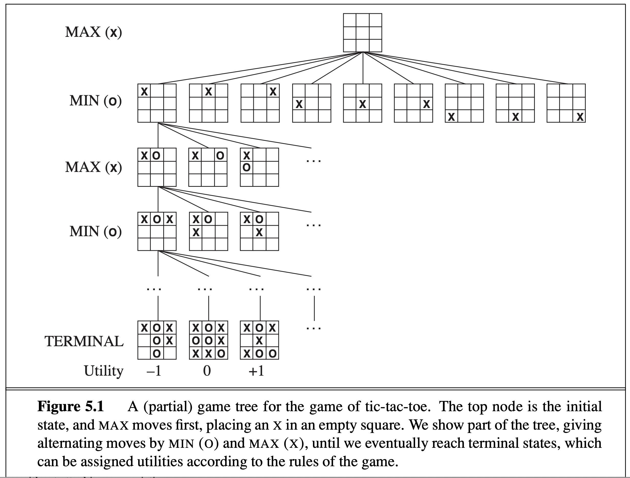
The above search algorithms are all about a single player. Now let’s look at game search such as chess where two players both play optimally. This type of search is called “adversarial search” or “minimax” search, where at odd levels (for you), you would maximize over the children nodes, but at even levels (for the opponent), you would minimize over the children nodes. This is the only way to guarantee that both players play optimally. At the leaf nodes, the score of each node, known as the “utility” is either +1 (if you win) or -1 (if you lose) or 0 (draw).
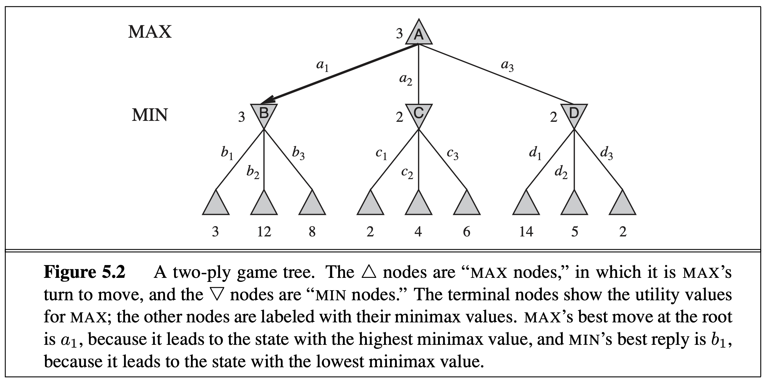
Here is another (abstract) example of minimax serach tree:
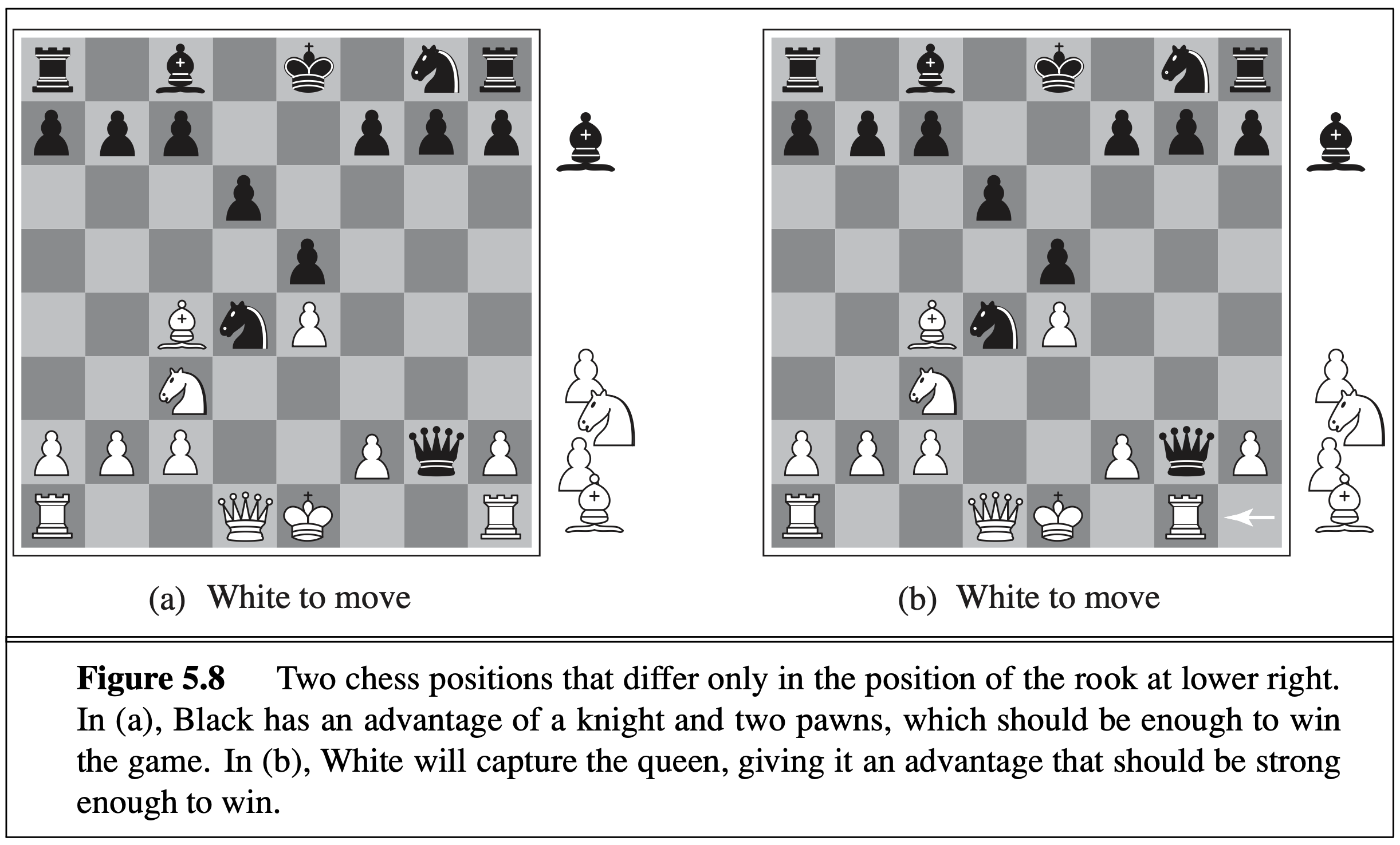
This type of search tree has big branching factors (think about how many moves are possible in a chess game state), so obviously for most games you can’t search till the leaf nodes (i.e., end of game). If you can only search for \(k\) levels (i.e., think ahead \(k\) steps), at the \(k\)th level, for a non-end game state, you need to estimate how likely you are going to win. This is the evaluation function, similar to the heuristic function in A* search. In chess, for example, we can write such a function based on the positions of pieces, based on our knowledge of chess.
To speed up the search, we cannot apply A* here because of the minimax, so AI scientists developed the super clever alpha-beta pruning algorithm to reduce the search space. The basic idea is to prune the branches that are guarantee not to influence the overall outcome, so that the search can be limited to more promising branches. To illustrate this with a real-life example, suppose somebody is playing chess, and it is their turn. Move “A” will improve the player’s position. The player continues to look for moves to make sure a better one hasn’t been missed. Move “B” is also a good move, but the player then realizes that it will allow the opponent to force checkmate in two moves. Thus, other outcomes from playing move B no longer need to be considered since the opponent can force a win. The maximum score that the opponent could force after move “B” is negative infinity: a loss for the player. This is less than the minimum position that was previously found; move “A” does not result in a forced loss in two moves.

Let’s consider the case for Chess (the most popular game in the West) and Go (the most popular game in East Asia). The branching factor of Chess (number of possible moves in a state) is orders of magnitude smaller than that of Go (which at open game is up to the size of the board, \(19\times 19=361\)), therefore, Chess is a much simpler search problem for AI. Indeed, AI Chess beat the World Champion in the 1990s (IBM Deep Blue vs. Kasparov), and it took AI much longer to do the same in Go. Since the search space is too prohibitive, classical methods like alpha-beta pruning does not work here, and scientists resorted to Monte-Carlo Tree Search. Another very hard problem for Go is the evaluation: unlike Chess where you can write a function based on piece positions (see above), here in Go, territory dominance is often ambiguous until the end game. So history needs to wait until the deep learning revolution (Unit 4) where we finally had the weaponry (convolutional neural networks, in Exploration 4.2) to do good estimation of winning likelihood. This, combined with deep reinforcement learning, finally gave AI Go the edge in 2016, when Google Deepmind AlphaGo beat World Champion Lee Se-dol.